Online Links:
Online Links:
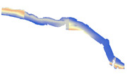
| Range of values | |
|---|---|
| Minimum: | 2.22045e-016 |
| Maximum: | .705603 |
  Taxa Model Formulas for GLM:
  Brittle Star
  taxa~Depth+I(Depth^2)+ Class+Block+Depth:Block, # Depth+ Depth^2+Class+Block+Depth:Block tryCatch(taxa33.glm <- glm(taxa~Depth+I(Depth^2)+
  Class+Block+Depth:Block, family=binomial(link="logit"), data=taxa.df),
  warning = function(x) { output.df[33,"flag"] <<- 1 }, finally = taxa33.glm <- glm(taxa~Depth+I(Depth^2)+ Class+Block+Depth:Block, family=binomial(link="logit"), data=taxa.df)
        )
  summary(taxa33.glm)

  MODEL SUMMARY:
  ==============

  Call:
  glm(formula = brit_in ~ Depth + I(Depth^2) + factor(Class) + factor(Block) + Depth:factor(Block), family = binomial(link="logit"), data = na.omit(d))

  Deviance Residuals:
  Min       1Q   Median       3Q      Max
  -1.5551  -0.6983  -0.4912  -0.1107   2.7408

  Coefficients:
                         Estimate Std. Error z value Pr(>|z|)
  (Intercept)          -1.6441219  0.6640992  -2.476  0.01330 *
  Depth                 0.1144813  0.0234621   4.879 1.06e-06 ***
  I(Depth^2)           -0.0013578  0.0002068  -6.567 5.13e-11 ***
  factor(Class)2       -0.9254904  0.3303862  -2.801  0.00509 **
  factor(Class)3       -0.8756778  0.5539213  -1.581  0.11391
  factor(Block)2       -1.5455724  0.5615242  -2.752  0.00591 **
  factor(Block)3       -4.4970380  0.7311817  -6.150 7.73e-10 ***
  Depth:factor(Block)2  0.0061871  0.0092539   0.669  0.50376
  Depth:factor(Block)3  0.0807144  0.0147237   5.482 4.21e-08 ***
  ---
  Signif. codes:  0 '***' 0.001 '**' 0.01 '*' 0.05 '.' 0.1 ' ' 1

  (Dispersion parameter for binomial family taken to be 1)

      Null deviance: 1009.10  on 922  degrees of freedom
  Residual deviance:  841.58  on 914  degrees of freedom
  AIC: 859.58

  Number of Fisher Scoring iterations: 5

  Analysis of Deviance Table

  Model: binomial, link: logit

  Response: brit_in

  Terms added sequentially (first to last)


                       Df Deviance Resid. Df Resid. Dev
  NULL                                   922    1009.10
  Depth                 1     2.14       921    1006.96
  I(Depth^2)            1    85.43       920     921.53
  factor(Class)         2     8.31       918     913.22
  factor(Block)         2    43.91       916     869.30
  Depth:factor(Block)   2    27.72       914     841.58
resampled to 10 meters
Krigsman, L.M., M.M. Yoklavich, E.J. Dick, and G.R. Cochrane (2012) Models and maps: predicting the distribution of corals and other benthic macro-invertebrates in shelf habitats. Ecosphere 3:1-16.
Online Links:
| Access_Constraints | None |
|---|---|
| Use_Constraints | USGS-authored or produced data and information are in the public domain from the U.S. Government and are freely redistributable with proper metadata and source attribution. Please recognize and acknowledge the U.S. Geological Survey and NOAA National Marine Fisheries as the originator(s) of the dataset and in products derived from these data. This information is not intended for navigation purposes. |
| Data format: | TIFF (version 9.3.1) Arcinfo grid Size: 887 |
|---|---|
| Network links: |
https://pubs.usgs.gov/ds/781/SantaBarbaraChannel/data/BrittleStars_SantaBarbaraChannel.zip https://pubs.usgs.gov/ds/781/SantaBarbaraChannel/data_catalog_SantaBarbaraChannel.html https://pubs.usgs.gov/ds/781/ |