Composite sidescan-sonar mosaic collected in Buzzards Bay by the U.S. Geological Survey offshore of Massachusetts in 2009, 2010, and 2011 (BB_backscatter1m.tif GeoTIFF image, UTM Zone 19N WGS84)

Metadata also available as - [Outline] - [Parseable text] - [XML]

Frequently anticipated questions:


What does this data set describe?

Title:
Composite sidescan-sonar mosaic collected in Buzzards Bay by the U.S. Geological Survey offshore of Massachusetts in 2009, 2010, and 2011 (BB_backscatter1m.tif GeoTIFF image, UTM Zone 19N WGS84)
Abstract:
These data were collected under a cooperative agreement between the Massachusetts Office of Coastal Zone Management (CZM) and the U.S. Geological Survey (USGS), Coastal and Marine Geology Program, Woods Hole Coastal and Marine Science Center (WHSC). Initiated in 2003, the primary objective of this program is to develop regional geologic framework information for the management of coastal and marine resources. Accurate data and maps of seafloor geology are important first steps toward protecting fish habitat, delineating marine resources, and assessing environmental changes due to natural or human impacts. The project is focused on the inshore waters of coastal Massachusetts, primarily in water depths of 5 to 30 meters (m) deep. Data collected for the mapping cooperative have been released in a series of USGS Open-File Reports (http://woodshole.er.usgs.gov/project-pages/coastal_mass/). The data collected in the study area in Buzzards Bay, Massachusetts, include high-resolution geophysics (bathymetry, backscatter intensity, and seismic reflection) and ground validation (sediment samples, video tracklines, and bottom photographs). The geophysical data are released in USGS Open-File Report 2012-1002, High-Resolution Geophysical Data from the Inner Continental Shelf: Buzzards Bay, Massachusetts (http://pubs.usgs.gov/of/2012/1002/). The sampling data have not been prepared for publication yet. The geophysical data were collected during four separate surveys conducted between 2004 and 2011 (National Oceanic and Atmospheric Administration (NOAA) survey H11319 (in 2004; bathymetry only) and USGS surveys 2009-002-FA, 2010-004-FA, and 2011-004-FA)) and cover 410 square kilometers of the inner continental shelf. More information about the individual USGS surveys conducted as part of the Buzzards Bay project can be found on WHCS Field Activity Web pages: 2009-002-FA: http://woodshole.er.usgs.gov/operations/ia/public_ds_info.php?fa=2009-002-FA 2010-004-FA: http://woodshole.er.usgs.gov/operations/ia/public_ds_info.php?fa=2010-004-FA 2011-004-FA: http://woodshole.er.usgs.gov/operations/ia/public_ds_info.php?fa=2011-004-FA Information about the NOAA survey can be found at: H11319: http://surveys.ngdc.noaa.gov/mgg/NOS/coast/H10001-H12000/H11319/DR/
  1. How might this data set be cited?
    U.S. Geological Survey, 2013, Composite sidescan-sonar mosaic collected in Buzzards Bay by the U.S. Geological Survey offshore of Massachusetts in 2009, 2010, and 2011 (BB_backscatter1m.tif GeoTIFF image, UTM Zone 19N WGS84): Open-File Report 2012-1002, U.S. Geological Survey, Coastal and Marine Geology Program, Woods Hole Coastal and Marine Science Center, Woods Hole, MA.

    Online Links:

    This is part of the following larger work.

    Ackerman, Seth D., Andrews, Brian D., Foster, David S., Baldwin, Wayne E., and Schwab, William C., 2013, High-Resolution Geophysical Data from the Inner Continental Shelf: Buzzards Bay, Massachusetts.: Open-File Report 2012-1002, U.S. Geological Survey, Reston, VA.

    Online Links:

  2. What geographic area does the data set cover?
    West_Bounding_Coordinate: -71.138008
    East_Bounding_Coordinate: -70.634536
    North_Bounding_Coordinate: 41.671438
    South_Bounding_Coordinate: 41.360841
  3. What does it look like?
    http://pubs.usgs.gov/of/2012/1002/GIS/browse_jpg/big/BB_backscatter1m.jpg (JPEG)
    Grey scale image of sidescan-sonar mosaic for Buzzards Bay, Massachusetts
  4. Does the data set describe conditions during a particular time period?
    Beginning_Date: 28-May-2009
    Ending_Date: 13-May-2011
    Currentness_Reference:
    ground condition of individual surveys on the following dates: 20090528-20090618; 20100515-20100520; 20110513
  5. What is the general form of this data set?
    Geospatial_Data_Presentation_Form: remote-sensing image
  6. How does the data set represent geographic features?
    1. How are geographic features stored in the data set?
      This is a Raster data set. It contains the following raster data types:
      • Dimensions 33600 x 41300 x 1, type Pixel
    2. What coordinate system is used to represent geographic features?
      Grid_Coordinate_System_Name: Universal Transverse Mercator
      Universal_Transverse_Mercator:
      UTM_Zone_Number: 19
      Transverse_Mercator:
      Scale_Factor_at_Central_Meridian: 0.999600
      Longitude_of_Central_Meridian: -69.000000
      Latitude_of_Projection_Origin: 0.000000
      False_Easting: 500000.000000
      False_Northing: 0.000000
      Planar coordinates are encoded using row and column
      Abscissae (x-coordinates) are specified to the nearest 1.000000
      Ordinates (y-coordinates) are specified to the nearest 1.000000
      Planar coordinates are specified in meters
      The horizontal datum used is D_WGS_1984.
      The ellipsoid used is WGS_1984.
      The semi-major axis of the ellipsoid used is 6378137.000000.
      The flattening of the ellipsoid used is 1/298.257224.
  7. How does the data set describe geographic features?
    BB_backscatter1m.tif.vat
    table associated with backscatter image (Source: Automatically generated by Esri software.)
    ObjectID
    Internal feature number. (Source: ESRI) Sequential unique whole numbers that are automatically generated.
    Value
    Backscatter Value. (Source: Cell values of the processed backscatter data) Automatically generated based on the backscatter value.
    Count
    Backscatter Value Count. (Source: Generated by ArcMap from the processed backscatter values) Automatically generated based on the number of cells in the image containing a particular backscatter value.
    Entity_and_Attribute_Overview:
    There are no attributes associated with a GeoTIFF image. Image pixel values contain acoustic reflectivity values normalized to an 8-bit data range (0-255) with the data range 1-253. Low-backscatter is represented by dark tones (low values) and high-backscatter is represented by bright tones (high values). The background color is set to 255 and can be turned off without removing data values.
    Entity_and_Attribute_Detail_Citation: U.S. Geological Survey

Who produced the data set?

  1. Who are the originators of the data set? (may include formal authors, digital compilers, and editors)
    • U.S. Geological Survey
  2. Who also contributed to the data set?
  3. To whom should users address questions about the data?
    Seth Ackerman
    U.S. Geological Survey
    Geologist
    384 Woods Hole Rd.
    Woods Hole, MA
    USA

    508-548-8700 x2315 (voice)
    508-457-2310 (FAX)
    sackerman@usgs.gov

Why was the data set created?

This GeoTIFF contains approximately 410 square kilometers of Klein 3000 sidescan-sonar data that were collected by the U.S. Geological Survey during three surveys (USGS surveys 2009-002-FA, 2010-004-FA and 2011-004-FA) offshore of Massachusetts, in Buzzards Bay. These data are used to define the seafloor composition and texture as part of the Massachusetts Seafloor Mapping Project.

How was the data set created?

  1. From what previous works were the data drawn?
    none (source 1 of 1)
    U.S. Geological Survey, Unpublished Material, raw backscatter data.

    Type_of_Source_Media: disc
    Source_Contribution:
    Data acquisition at sea: Sidescan sonar data were collected with a Klein 3000 dual frequency (132/445 kHz) sidescan-sonar towfish on the M/V Megan T. Miller (2009-002-FA and 2010-004-FA) and the M/V Scarlett Isabella (2011-004-FA). During all three surveys the sonar was towed from the stern A-frame of the vessel. A 3PS digital block cable counter was used to measure the amount of tow cable deployed, and cable out values were transmitted via serial connection to the SonarPro acquisition software (versions 10.0 and 11.0) for layback calculation. Tracklines are generally spaced 100m apart with a swath width of 200m (spaced 150m apart with a swath width of 300m in the central Buzzards Bay area where the USGS data overlaps with NOAA multibeam echo-sounder data). Most of the data were acquired roughly parallel to the axis and shipping lane within Buzzards Bay at an average speed of 5 knots. Some survey specific specifications are listed below: 2009-002-FA SonarPro version: 10.0 nav: from the antenna on the aft end of the acquisition van into the Ashtech BRG2 receiver (DGPS) sheave offsets x: -2.0m; y:-8.35m; z:+2.0m 2010-004-FA SonarPro version 11.0 nav: from the center antenna on the SWATHplus pole into the NovAtel DL-V3 receiver (RTK) sheave offsets x:-4.1m; y:-14.94m; z:-1.33m 2011-004-FA SonarPro version 11.0 nav: from the antenna on the fwd end of the acquisition van into the Ashtech BRG2 receiver (DGPS) sheave offsets x: +4.31m; y:-9.18m; z:0.0m
  2. How were the data generated, processed, and modified?
    Date: 2011 (process 1 of 8)
    XSonar (versions: 1.1 in 2009 and 2.0 in 2010 and 2011) was used to apply a median filter (4 pixels across track by 3 pixels along track) to the raw sidescan-sonar data (XTF) to remove speckle noise. The data were further processed to correct fish altitudes, reduce slant-range and beam-angle distortions, and merge navigation (Danforth, 1997). Adjacent sidescan sonar lines were mapped out separately from XSonar into north-heading and south-heading sonar mosaics at 1 meter/pixel resolution. Sidescan areas were defined within the survey trackline planning scheme such that the sonar images mapped in XSonar would have the same line orientation and keep the working mosaics to a manageable filesize.
    
    
    Below are the typical parameters for processing with XSonar:
    
    
    File Type:
    
    
    XTF, Low Frequency (132 kHz)
    
    
    Setup Option:
    
    
    Navigation= Lat/Lon
    
    
    Navigation Interval= 1 minute
    
    
    Demultiplexing Range and Filter options:
    
    
    Across track=4 (pixels) Along track= 3 (pixels)
    
    
    Port/Starboard Normalize = 4095 (default)
    
    
    Port High Pass: 65535 (default)
    
    
    Input= 16 bit
    
    
    Normalize Image= yes.
    
    
    Beam Pattern Correction options:
    
    
    Number of lines= 90
    
    
    Ping overlap=45
    
    
    Max beam angle= 90 (default)
    
    
    Response angle=55 (default)
    
    
    Data normalization (0-255)=1 (default)
    
    
    Port/Stbd Tone Adjustment= "on" and "Normal"
    
    
    Processing occurred in 2009, 2010, and 2011. Person who carried out this activity:
    Seth Ackerman
    U.S. Geological Survey
    Geologist
    384 Woods Hole Rd.
    Woods Hole, MA

    (508) 548-8700x2315 (voice)
    (508) 457-2310 (FAX)
    sackerman@usgs.gov
    Date: 2011 (process 2 of 8)
    A PCI Geomatica (versions: 10.0.3 (in 2009) and 10.1 (2010,2011)) project was created for each subarea of the Buzzards Bay survey area. The north and south-heading working mosaics from the previous process step were imported into PCI Geomatica to be digitally mosaicked using PCI's OrthoEngine and procedures described in Paskevich (1996). The mosaicking process produces an enhanced, geographically correct, sidescan-sonar mosaic with 1 meter/pixel resolution. The Buzzards Bay survey area was divided into six subareas to maintain reasonable file sizes and processing time. The subareas were then mosaicked together into a composite backscatter image for the entire survey area. The composite mosaic was exported as a GeoTIFF image. Processing occurred in 2009, 2010, and 2011. Person who carried out this activity:
    Seth Ackerman
    U.S. Geological Survey
    Geologist
    384 Woods Hole Rd.
    Woods Hole, MA

    (508) 548-8700x2315 (voice)
    (508) 457-2310 (FAX)
    sackerman@usgs.gov
    Date: 2011 (process 3 of 8)
    While most NODATA pixels in the GeoTIFF image (outside the survey bounds) have backscatter values of 255, some were assigned values of 254 during the mosaicking process. Adobe Photoshop CS4 (version 11.0) was used to select all of the NODATA pixels and assign the single NODATA value of 255. All backscatter data within the survey area have values of less than 255, but some small data gaps (NODATA) do occur. Person who carried out this activity:
    Seth Ackerman
    U.S. Geological Survey
    Geologist
    384 Woods Hole Rd.
    Woods Hole, MA

    (508) 548-8700x2315 (voice)
    (508) 457-2310 (FAX)
    sackerman@usgs.gov
    Date: 2012 (process 4 of 8)
    A TIFF World File (TFW) was created using Mentor Software GeoTiffExaminer (no version) to define the spatial extent of the TIFF image. GeoTiffExaminer was also used to transfer the spatial information to the TIFF, creating a GeoTIFF image Person who carried out this activity:
    Seth Ackerman
    U.S. Geological Survey
    Geologist
    384 Woods Hole Rd.
    Woods Hole, MA

    (508) 548-8700x2315 (voice)
    (508) 457-2310 (FAX)
    sackerman@usgs.gov
    Data sources used in this process:
    • BB_backscatter1m.tfw
    Data sources produced in this process:
    • BB_backscatter1m.tif
    Date: 08-Dec-2015 (process 5 of 8)
    Edits to the metadata were made to fix any errors that MP v 2.9.32 flagged. This is necessary to enable the metadata to be successfully harvested for various data catalogs. In some cases, this meant adding text "Information unavailable" or "Information unavailable from original metadata" for those required fields that were left blank. Other minor edits were probably performed (title, publisher, publication place, etc.). The distribution format name was modified in an attempt to be more consistent with other metadata files of the same data format. The metadata date (but not the metadata creator) was edited to reflect the date of these changes. The metadata available from a harvester may supersede metadata bundled within a download file. Compare the metadata dates to determine which metadata file is most recent. Person who carried out this activity:
    U.S. Geological Survey
    Attn: VeeAnn A. Cross
    Marine Geologist
    384 Woods Hole Rd
    Woods Hole, MA

    508-548-8700 x2251 (voice)
    508-457-2310 (FAX)
    vatnipp@usgs.gov
    Date: 20-Jul-2018 (process 6 of 8)
    USGS Thesaurus keywords added to the keyword section. Person who carried out this activity:
    U.S. Geological Survey
    Attn: VeeAnn A. Cross
    Marine Geologist
    384 Woods Hole Road
    Woods Hole, MA

    508-548-8700 x2251 (voice)
    508-457-2310 (FAX)
    vatnipp@usgs.gov
    Date: 18-Nov-2019 (process 7 of 8)
    Crossref DOI link was added as the first link in the metadata. Person who carried out this activity:
    U.S. Geological Survey
    Attn: VeeAnn A. Cross
    Marine Geologist
    384 Woods Hole Road
    Woods Hole, MA

    508-548-8700 x2251 (voice)
    508-457-2310 (FAX)
    vatnipp@usgs.gov
    Date: 08-Sep-2020 (process 8 of 8)
    Added keywords section with USGS persistent identifier as theme keyword. Person who carried out this activity:
    U.S. Geological Survey
    Attn: VeeAnn A. Cross
    Marine Geologist
    384 Woods Hole Road
    Woods Hole, MA

    508-548-8700 x2251 (voice)
    508-457-2310 (FAX)
    vatnipp@usgs.gov
  3. What similar or related data should the user be aware of?
    Danforth, W.W., O'Brien, T.F., and Schwab, W.C., 1991, USGS image processing system: near real-time mosaicking of high-resolution sidescan-sonar data: Sea Technology Jan. 1991, Sea Technology, Arlington, VA.

    Danforth, William W., 1997, XSonar/ShowImage: A complete system for rapid sidescan-sonar processing and display.: Open-File Report 97-686, U.S. Geological Survey, Reston, VA.

    Paskevich, Valerie, 1996, MAPIT: An improved method for mapping digital sidescan sonar data using the Woods Hole Image Processing System (WHIPS) Software: Open-File Report 96-281, U.S. Geological Survey, Reston, VA.


How reliable are the data; what problems remain in the data set?

  1. How well have the observations been checked?
    Image pixel values contain acoustic reflectivity values normalized to an 8-bit data range (0-255). Low-backscatter is represented by dark tones (low values) and high-backscatter is represented by bright tones (high values). The nodata value is 255.
  2. How accurate are the geographic locations?
    Field activity 2009-002: The Klein 3000 was towed from the stern A-frame of the M/V Megan T. Miller. Differential GPS (DGPS) position data were provided by the Ashtech BRG2 receiver and recorded to the raw data files (XTF) via SonarPro (version 10.0) on the sonar acquisition computer. The GPS antenna was mounted on the aft end of the acquisition lab van. All GPS data during this survey was referenced to the WGS84 horizontal datum. The horizontal offsets between the GPS antenna and the sheave on the A-frame were measured prior to the survey (x: -2.0m; y: -8.35m; z: +2m). The side-scan tow cable was deployed through a 3PS digital block cable counter attached to the A-frame. Real-time cable-out measurements were transmitted via serial connection to the SonarPro acquisition software, which calculated tow-fish layback. All horizontal offsets were applied in the acquisition software so the navigation recorded in the XTF data reflect the position including the layback offset. The layback calculations do not account for fish motion behind the vessel, which is caused by sea state and vessel speed induced changes in the angle and scope of the tow cable. DGPS positional accuracy is estimated to be within 3-5 m; WAAS enable DGPS is estimated to be less than 3 m. Taking the additional fish motion and cable movement into account, as well as the mosaicking process, the positional accuracy for this dataset is estimated to be within 30 m. The Klein 3000 was towed from the stern A-frame of the M/V Megan T. Miller. Real-Time Kinematic (RTK) GPS position data were provided by the NovAtel DL-V3 receiver and recorded to the raw data files (XTF) via SonarPro (version 11.0) on the sonar acquisition computer. The GPS antenna was mounted on the top of the SWATHplus (interferometric bathymetry) transducer pole, midship on the starboard side (the middle of the 3 bathymetry system antennas). On a few brief occasions the RTK-GPS signal was lost and the navigation system fell back to standalone DGPS or GPS mode. In these cases, the lower quality positions were used and no corrections were made for RTK navigation gaps. All GPS data during this survey were referenced to the WGS84 horizontal datum. The horizontal offsets between the GPS antenna and the sheave on the A-frame were measured prior to the survey (x: -4.1m; y: -14.94m; z: -1.33m). The side-scan tow cable was deployed through a 3PS digital block cable counter attached to the A-frame. Real-time cable-out measurements were transmitted via serial connection to the SonarPro acquisition software, which calculated tow-fish layback. All horizontal offsets were applied in the acquisition software so the navigation recorded in the XTF data reflect the position including the layback offset. The layback calculations do not account for fish motion behind the vessel, which is caused by sea state and vessel speed induced changes in the angle and scope of the tow cable. RTK positional accuracy is estimated to be less than 1 m. Taking the additional fish motion, cable movement and RTK-GPS navigation dropouts into account, as well as the mosaicking process, the positional accuracy for this dataset is estimated to be within 30 m. Field activity 2011-004: The Klein 3000 was towed from the stern A-frame of the M/V Scarlett Isabella. Differential GPS (DGPS) position data were provided by the Ashtech BRG2 receiver and recorded to the raw data files (XTF) via SonarPro (version 11.0) on the sonar acquisition computer. The GPS antenna was mounted on the forward end of the acquisition lab van. All GPS data during this survey was referenced to the WGS84 horizontal datum. The horizontal offsets between the GPS antenna and the sheave on the A-frame were measured prior to the survey (x: +4.31m; y: -9.18m; z: 0.0m). The side-scan tow cable was deployed through a 3PS digital block cable counter attached to the A-frame. Real-time cable-out measurements were transmitted via serial connection to the SonarPro acquisition software, which calculated tow-fish layback. All horizontal offsets were applied in the acquisition software so the navigation recorded in the XTF data reflect the position including the layback offset. The layback calculations do not account for fish motion behind the vessel, which is caused by sea state and vessel speed induced changes in the angle and scope of the tow cable. DGPS positional accuracy is estimated to be within 3-5 m; WAAS enable DGPS is estimated to be less than 3 m. Taking the additional fish motion and cable movement into account, as well as the mosaicking process, the positional accuracy for this dataset is estimated to be within 30 m.
  3. How accurate are the heights or depths?
  4. Where are the gaps in the data? What is missing?
    Only the subset of sidescan-sonar backscatter data collected within the Buzzards Bay study area during field activities 2009-002-FA, 2010-004-FA and 2011-004-FA are included in this spatial dataset. Approximately 340 square-km of additional sidescan-sonar backscatter data collected within Vineyard Sound, Massachusetts during these field activities were published in USGS Open-File Report 2012-1006 High-Resolution Geophysical Data from the Inner Continental Shelf: Vineyard Sound, Massachusetts (http://pubs.usgs.gov/of/2012/1006/). Some sections of sonar data with excess noise were clipped during processing.
  5. How consistent are the relationships among the observations, including topology?
    This image represents sidescan-sonar backscatter data collected along the main survey lines; backscatter data was typically not collected along the tieline survey lines and therefore there is no crossline data included in this image. Gaps may occur along-track and between adjacent lines, especially where the ship had to maneuver to avoid obstacles during surveying.

How can someone get a copy of the data set?

Are there legal restrictions on access or use of the data?
Access_Constraints None
Use_Constraints Public domain data from the U.S. Government are freely redistributable with proper metadata and source attribution. Please recognize the U.S. Geological Survey as the originator of the dataset.
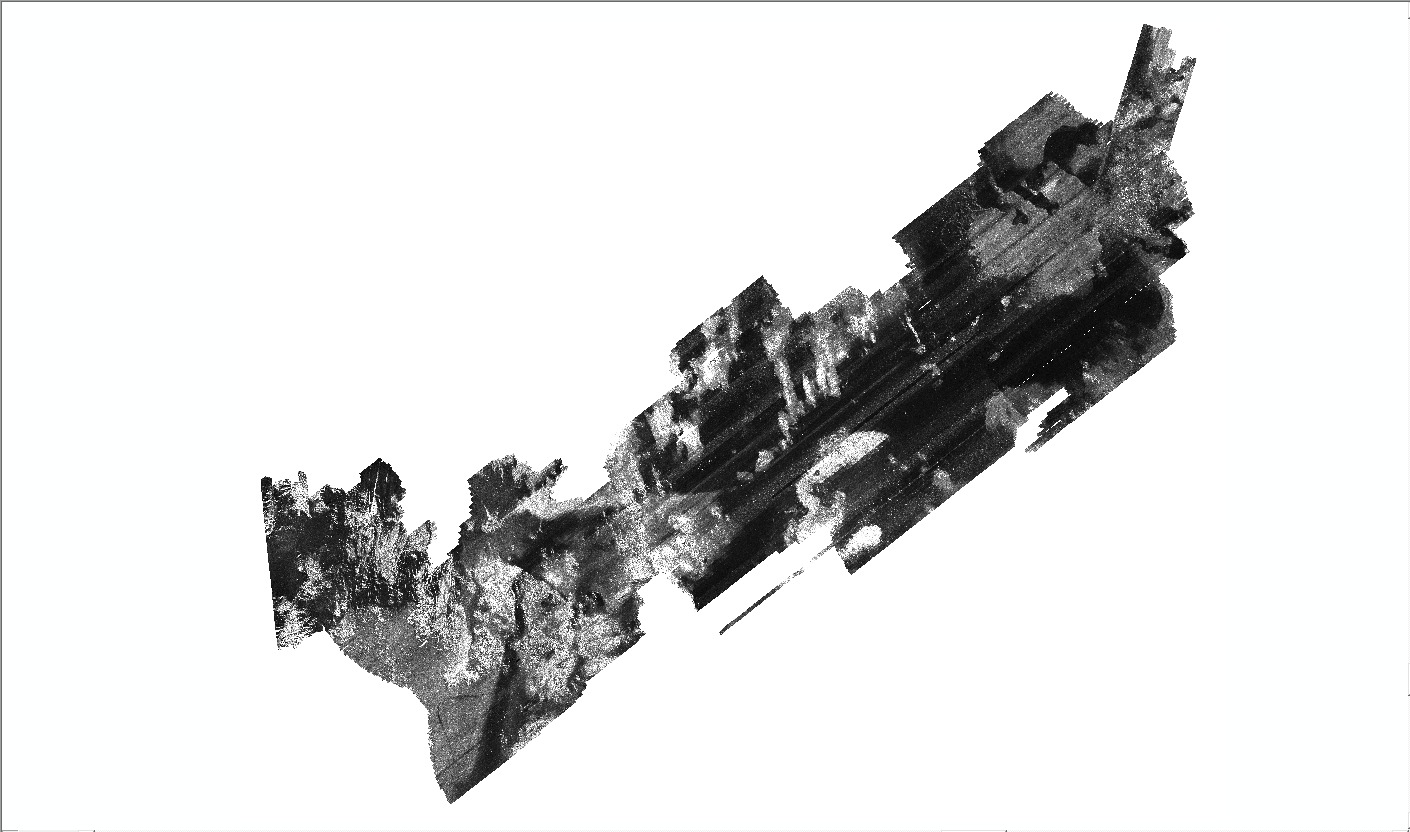
  1. Who distributes the data set? (Distributor 1 of 1)
    Seth Ackerman
    U.S. Geological Survey
    Geologist
    384 Woods Hole Rd.
    Woods Hole, MA
    USA

    508-548-8700 x2315 (voice)
    508-457-2310 (FAX)
    sackerman@usgs.gov
  2. What's the catalog number I need to order this data set? Downloadable Data
  3. What legal disclaimers am I supposed to read?
    Neither the U.S. Government, the Department of the Interior, nor the USGS, nor any of their employees, contractors, or subcontractors, make any warranty, express or implied, nor assume any legal liability or responsibility for the accuracy, completeness, or usefulness of any information, apparatus, product, or process disclosed, nor represent that its use would not infringe on privately owned rights. The act of distribution shall not constitute any such warranty, and no responsibility is assumed by the U.S. Geological Survey in the use of these data or related materials. Any use of trade, product, or firm names is for descriptive purposes only and does not imply endorsement by the U.S. Government.
  4. How can I download or order the data?
    • Availability in digital form:
      Data format: This zip (WinZip v. 14.0) file contains a geographic GeoTIFF image of side-scan sonar data from the Buzzards Bay survey area. This also includes a TIFF World File (tfw) and associated metadata. in format GeoTIFF (version Information unavailable from original metadata.) Size: 330
      Network links: http://pubs.usgs.gov/of/2012/1002/GIS/raster/backscatter/BB_backscatter1m.zip
      Media you can order: DVD-ROM (Density 4.75 GB) (format UDF)
    • Cost to order the data: none

  5. What hardware or software do I need in order to use the data set?
    This zip file contains a GeoTIFF image with an accompanying world file. To utilize this data, the user must have an image viewer, image processing or GIS software package capable of importing a GeoTIFF image. A free spatial data viewer, ArcExplorer, capable of displaying the data is available from Esri at www.esri.com. The zip file also contains associated metadata.

Who wrote the metadata?

Dates:
Last modified: 18-Mar-2024
Metadata author:
Seth Ackerman
U.S. Geological Survey
Geologist
384 Woods Hole Rd.
Woods Hole, MA
USA

508-548-8700 x2315 (voice)
508-457-2310 (FAX)
whsc_data_contact@usgs.gov
Contact_Instructions:
The metadata contact email address is a generic address in the event the person is no longer with USGS. (updated on 20240318)
Metadata standard:
FGDC Content Standards for Digital Geospatial Metadata (FGDC-STD-001-1998)

This page is <https://cmgds.marine.usgs.gov/catalog/whcmsc/open_file_report/ofr2012-1002/bb_backscatter1m.tif.faq.html>
Generated by mp version 2.9.51 on Mon Mar 25 16:05:40 2024