
lResearch civil engineer, U.S. Geological Survey, 345 Middlefield Road, Menlo Park, CA 94025.
2Research geologist, U.S. Geological Survey, 345 Middlefield Road, Menlo Park, CA 94025
REFERENCE: Kayen, R. E., Edwards, B. D., and Lee, H. J., "Nondestructive Laboratory Measurement of Geotechnical and Geoacoustic Properties Through Intact Core-Liner," Nondestructive and Automated Testing for Soil and Rock Properties, ASTM STP 1350, W. A. Marr and C. E. Fairhurst, Eds., American Society for Testing and Materials, West Conshohocken, PA, 1999.
Abstract
USGS Multi-SensorCore Logger
Calibrations
System Quality Assurance and Quality Control
Case Study: Non-invasive Property Determination for Environmental Study of the Seafloor
Conclusions
Acknowledgments
References
automation, bulk density, core liner, geotechnical, geoacoustic, Lambert attenuation, logger, robotics, sediment, soil, p-wave, sound velocity
Numerous investigations of the coastal zone, lake floor, and seafloor by the USGS involve the sampling of soil retained in metal or plastic liners. Soil samples are taken by the USGS to address topics such as assessment of liquefaction and landsliding during earthquakes, identification of regions of the seafloor contaminated by human activities, understanding the history of sedimentation and climate change preserved in the sediment record, and evaluation of mineral resource potential. For carefully sampled and stored sediment, intrinsic sediment properties (e.g., grain size) generally remain unchanged after sampling, whereas, sediment state properties can be highly susceptible to change. State properties include those altered by volumetric changes in pore water, orby accumulated strain (e.g., density, velocity, strength, and their related moduli). Even for carefully sampled soil, state properties can be significantly altered during storage, transportation, extrusion and laboratory testing.
To better estimate the in-place properties of such soil samples we prefer to nondestructively measure the state properties by use of a custom designed and built logging device used to scan sediment cores nondestructively. Our device measures three soil properties: 1) soil compression wave (p-wave) velocity; 2) soil wet bulk-density by Lambert; 3) and sediment magnetic susceptibility. This paper describes our methodology for measuring soil p-wave velocity and bulk density, two properties useful to geotechnical engineers for site characterization. We omit measurement of magnetic susceptibility in the discussion because it is an intrinsic property generally not useful to engineers.
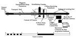
Field sampling operations, both onshore and in the subaqueous environment typically focus on collecting soil samples with a variety of borehole or coring devices. Recovered samples are encased in liner tube and logged for their geotechnical and geoacoustic properties on the USGS multi-sensor whole core sediment-logging device, built in Great Britain by Geoteck, Ltd. Sealed cylindrical sediment cores are placed horizontally upon a transport sled and moved by a computer-controlled stepper motor through a frame supporting three sensors (Figure 1). In a sequence, the logging device measures core diameter and p-wave travel time to compute p-wave velocity, attenuation of gamma rays from a 137Cs source to compute soil wet bulk density; and magnetic susceptibility of soil particles via a magnetic field hoop. Measurements of velocity, density, and magnetic susceptibility are typically taken at 1-centimeter increments, often within the first hour after the cores are sampled. The transport sled is capable of carrying individual core sections up to 1.5 meters in length.
Figure 1: Plan view diagram of the USGS multi-sensor core sediment logging device and computer system. Click on figure for larger image (27K).
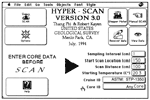
The USGS developed an Apple HyperTalkTM driven software program called HYPERSCAN to automate the logger system and support a number of user and system tailored scanning options (Kayen and Phi 1997). We chose the Macintosh interface to create an intuitive mouse/button-driven environment so that a laboratory technician could easily acquire data (Figure 2). The program includes a suite of sub-routines for system calibration and permits the sensors to be activated or disabled. For example, cores retained within metal core liner (e.g. Shelby tube samples) do not allow for measurement of magnetic properties: in this case we can disable the magnetic susceptibility sensor to increase the efficiency of the system. Computer automation also allows the technician to maintain some physical distance from the cesium (137Cs) gamma ray source. During automated scanning, an unsplit sediment core is driven down a track system in user-prescribed increments and the Macintosh computer interrogates sensors. As data enter the computer, the bulk density, p-wave velocity, and magnetic susceptibility are calculated, logged into a matrix data file, and presented in real-time on a 3-plot graphics display window.
Figure 2: USGS graphical user-interface (GUI) developed for the multi-sensor logging device, written in the Apple Macintosh HYPERTALKTM programming language (Kayen and Phi, 1997). The buttons activate sub-routines for help assistance; calibration routines; and scan modes. Click on figure for larger image (52K).
Compression- Wave Velocity
The compression wave velocity, Vp, of sediment is calculated from the measured core diameter and wave-travel time, correcting for the liner thickness, electronic signal delays associated with the travel-time within the transducer head, and core liner travel-time. In our core logger system, a transmitter and receiver transducer sit opposite one another and orthogonal to the direction of core motion (Figure 1). Spring-loaded transducer heads are used to couple the sensors to the core liner. Water is sprayed between the core liner and transducers to improve the acoustic-coupling, usually resulting in transmission of a strong and well-defined p-wave trace. Linear displacement transducers (LVDT) are mounted on the acoustic transducers and used to determine the diameter of the core passing through the sensors. The total travel-time, t, of a p-wave pulse sent through a sediment core by transmitting and receiving transducers is as follows:
t = ttransrnitter-delay + 2tliner + tsediment+ treceiver-delay (1)
The travel path length through the soil is D-21, so the velocity of the sediment can be determined by subtracting transducer delays and the transmission time through the liner. The transducer delay is determined by directly coupling the transmitting and receiving transducer heads and measuring the p-wave travel time. The one remaining variable, the travel time through the 2 liner walls, is determined as the value that brings the velocity of the distilled water standard to 1491.7 m/sec at 23ºC. Compression wave velocity of soil is calculated as:
![]() (2)
(2)
The pore-water salinity, temperature, total confining pressure, and soil bulk density affect the p-wave velocity of soil. Standards for correcting velocity measurements to a common reference state require reporting of velocities at laboratory conditions of 1-atm pressure and 23ºC (Hamilton and Bachman 1982). Temperature corrections are made using equation 3, regressed from standard correction tables (U.S. Naval Oceanographic Office 1962).
![]() (3)
(3)
Where Vp-23º is the corrected velocity in meters/sec., Vp-Tº is the velocity calculated at the measured temperature, and Tmeas. is the laboratory measured soil temperature in ºC. Calibration of sound speed through the distilled water-filled core standard is made simultaneously with the density calibration.
Wet Bulk Density
Bulk density is the ratio of the total soil weight, to the soil volume. The configuration of our device allows for a core to pass between a scintillation counter and a vessel emitting a one-centimeter columnated beam of gamma rays from a radioisotope Cesium-137 source. Sediment bulk density (![]() b) is calculated from the gamma ray attenuation characteristics of the cores according to Lambert's law. For a user-defined time period, the number of gamma decays emitted from the Cesium-vessel, passing through the core and received at the scintillation detector is counted. To address the health and safety concerns of technicians and satisfy the requirements of our radiation use permits and NRC license, we use lead shielding to reduce the amount of gamma ray emission away from the scintillation counter sensor to nearly background levels.
b) is calculated from the gamma ray attenuation characteristics of the cores according to Lambert's law. For a user-defined time period, the number of gamma decays emitted from the Cesium-vessel, passing through the core and received at the scintillation detector is counted. To address the health and safety concerns of technicians and satisfy the requirements of our radiation use permits and NRC license, we use lead shielding to reduce the amount of gamma ray emission away from the scintillation counter sensor to nearly background levels.
The number of scintillation's transmitted from the source to the scintillation counter through air, is referred to as the unattenuated gamma count, Io. For the case where a homogeneous material of some thickness, d, lies between the Cesium source and sensor, the attenuated gamma ray count, I, can be related to the unattenuated number of gamma decays, Io, the material thickness, d, the soil bulk density, ![]() b, and the soil Compton scattering coefficient, µ1, 2) by Lambert's Law (CRC 1969):
b, and the soil Compton scattering coefficient, µ1, 2) by Lambert's Law (CRC 1969):
I = Io exp {-µs  bd} (4)
The bulk density of the soil can be determined as follows:
 (5)
(5)
For recovered whole sediment cores encased in liners, we must account for the influence of the core-liner to get an accurate estimation of the soil density. The liner correction accounts for liner attenuation of the gamma-ray beam through absorption and scattering, effects controlled by 1) the liner Compton scattering coefficient,µ1, 2) liner wall thickness, 1, and 3) liner wall density, ![]() 1. For sediment contained within a core liner of outer diameter, D, and double-wall thickness, 21, equation (5) can be rewritten as:
1. For sediment contained within a core liner of outer diameter, D, and double-wall thickness, 21, equation (5) can be rewritten as:
 (6)
(6)
Equation 6 relates the attenuated gamma-ray count to the partial scattering influences of the liner and soil, and can be used to assess the density of material contained within a variety of liner-types, both plastic and metal. To determine the bulk density of soil, equation 6 must first undergo transformation to base-e logarithm.
 (7)
(7)
Density measurements of soil contained within intact core-liner are calibrated to the known standards of water (![]() w=1.00 g/cc) and aluminum (
w=1.00 g/cc) and aluminum ( ![]() al=2.70 g/cc). These two standards serve as end-members that fully-bound the limits of soil density. The added advantage of using these materials is that their respective Compton scattering coefficients, µw and µal, are similar to those of soil pore water and soil alumina-silicate particles, although we determine these parameters empirically. To account for the influence of the liner, a water-aluminum standard is prepared by inserting a solid-cylinder of 6250 or 1100F aluminum into an unsplit section of core-liner identical to the liner used for soil sampling. The length of milled aluminum fills one-half the total length of the "calibration standard"-core-liner and distilled water fills the remaining portion. Caliper measurements of the liner diameter and wall thickness are made to determine the travel path-length through the liner and interior space.
al=2.70 g/cc). These two standards serve as end-members that fully-bound the limits of soil density. The added advantage of using these materials is that their respective Compton scattering coefficients, µw and µal, are similar to those of soil pore water and soil alumina-silicate particles, although we determine these parameters empirically. To account for the influence of the liner, a water-aluminum standard is prepared by inserting a solid-cylinder of 6250 or 1100F aluminum into an unsplit section of core-liner identical to the liner used for soil sampling. The length of milled aluminum fills one-half the total length of the "calibration standard"-core-liner and distilled water fills the remaining portion. Caliper measurements of the liner diameter and wall thickness are made to determine the travel path-length through the liner and interior space.
During the density calibration, the numbers of scintillation's-per-second are logged for transmission of gamma rays through air to give a measure of Io. Similar measurements are made for the "calibration standard" to determine the scintillation count for water-filled liner, Iw, and aluminum-filled liner, Ial. We determine the attenuation ratios for water and aluminum ( Io/ Iw and Io/Ial) and solve for the remaining unknowns, µ11 and µs, by setting up two simultaneous equations and eliminating one of the variables. For each soil-core, we scan the whole-round sections using the same Compton scattering parameters that correct the calibration-standards water and aluminum to their known values of density.
Calibration standards are run repeatedly during testing programs. Typically, to calibrate the sediment-core profiles for density, measurements are made from our calibration-standard after every core is logged on our device. The empirical Compton scattering coefficient for soil that is determined by this method tends to be approximately 40% lower than the published value for water, and at present the reason for this is unknown. The circular cross-section of soil cores, as compared with an idealized tabular cross-section may be the cause of the lower µs, and future experiments are planned to assess the influence of core liner geometry on the scattering of gamma-rays.
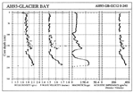
After system calibration is complete, soil cores are run through the logger system and calibration corrected densities and velocities are presented, along with magnetic susceptibility, on a real-time graphics display. Typical run-time for driving a 150 centimeter core through the sensor array is approximately 35 minutes. An example of output data from the USGS logger is presented in Figure 3. The resultant high-resolution measurements at 1 cm spacing clearly delineate two fining-upward sequences within the core section at depths greater than 95 cm that are interpreted to be sandy-turbidite deposits buried beneath finer-grained glacial mud. Manual acquisition of these data through destructive laboratory testing for density, velocity, and magnetics would take approximately one man-week per core. The USGS logger system scanned this 240 cm core in three sections in approximately one-hour.
Figure 3: Example data from the USGS whole core sediment logging device. Click on figure for larger image (56K).
Several approaches are taken to assess the quality of our non-invasive measurements of bulk density and sound speed velocity through a core-liner. After extensive use of our system at sea and in our shore-based laboratory, several hundred calibration log files containing 30 or more data points were separated into individual files for water-filled and aluminum-filled core-liner. These material dependent sub-sets of the calibration files were then used to calculate the mean and standard deviation for the measured density and velocity and compared with the known values for water and aluminum presented in parenthesis (Table 1).
Table 1: Data quality for gamma-ray bulk density and sound speed
(Known values are shown in parentheses).
| Density and Velocity Statistics | Distilled Water | Aluminum |
| Mean Density (g/cc) (Known b) |
1.004 (1.00) |
2.700 (2.70) |
| Density Std. Dev. (g/cc) | 0.010 | 0.016 |
| Mean Velocity (Km/sec) (Known Vp) |
1.4910 (1.4917) |
unknown |
| Velocity Std. Dev. (Km/sec) | 0.0024 | unknown |
The mean value of the calculated and measured density of distilled water was within 0.4% of the known value and the mean value for aluminum was exactly the known value. It was found that the standard deviation for density measurements is on the order of 0.6-1.0% of the measured value. The mean-measured sound speed. for distilled water at 23ºC was within 0.05% of the known value, and standard deviation of the distilled water velocity measurements is 0.16% about the mean measured value. The value of sound speed through aluminum is, at present, unknown. These statistic data indicate the very high accuracy and repeatability of the USGS multi-logger system.
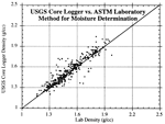
Subsequently, sediment samples are taken from opened sections of cores after logging, and moisture contents are calculated using standard procedures presented by the American Society of Testing and Materials (ASTM) and procedures developed at the USGS for the determination of water content of marine sediment. A comparison between USGS multi-logger derived-densities and laboratory determined densities (converted from moisture content values using an assumed grain specific gravity of 2.65 and saturation of 100%) for approximately the same depth in the core is presented in Figure 4. The data generally fall around the line of unity with scatter about a line of perfect correlation (R=1). The scatter is, most likely, attributable to errors in sampling the exact depth interval scanned by the logging device, to the different nature of the two density measurements, and the assumed value of specific gravity. The logging system beams gamma rays across the entire core section and thereby determines a bulk average density representative of the entire mass of the increment. The laboratory estimate is made from a discrete sample taken near the center of the core section, having a mass of approximately 5 grams. Thus, discrete physical samples may not be representative of the average whole section density if lateral inhomogeneities exist. For example, if a thick remolded zone occurs along the inside of the liner wall, the laboratory measurement taken at the center of the core may be more representative of the field conditions and preferable to the logger estimate. On the other hand, for non-cohesive material, drainage of pore water during physical sampling may result in an alteration of the density state. These concerns serve to reinforce the importance of taking high quality core samples and supporting non-invasive measurements of density with physical measurements from sample core sections.
Figure 4: Comparison of USGS logger densities and densities estimated by the ASTM standard prodecure for soil moisture determination. Click on figure for larger image (36K).
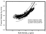
The relation between sound speed and sediment bulk density is constrained by the compressibility of the pore water and mineral structure, and the shear (rigidity) modulus of the sediment (Hamilton 1971). In an exhaustive study of continental terrace (shelf and slope) material from margins around the world, Hamilton and Bachman (1982) proposed a regression equation that predicts sound speed as a function of bulk density for typical terrace material. Hamilton (1971) and Hamilton and Bachman (1982) measured sound speed and bulk density directly in the laboratory from ~10 cm tall sediment sub-samples using a destructive technique. We compared the equation of Hamilton and Bachman (1982) with a sub-set of data (approximately 25-thousand data points) from one USGS offshore sampling cruise on the California continental margin between San Francisco and San Diego (Figure 5). The data collected by the USGS core sediment logging system fall generally within the ±1 standard deviation bounds of their equation, although the curvature of the data set is somewhat less than that of the predictor equation for moderate to high densities typical of non-cohesive materials. The difference in curvature is probably attributable to the relative richness of the Hamilton and Bachman data set, collected from numerous margins and varied mineralogic source provenances. Nevertheless, the reasonably good regression fit to the USGS logger data indicates that we are accurately measuring bulk density and sound speed in whole core sections in a nondestructive manner and can account for, and eliminate, the influence of the core liner on our measurements.
Figure 5: Field data from USGS cruise F2-92-SC and the relation proposed by Hamilton and Bachman (1982). Click on figure for larger image (32K).
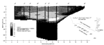
The County of Los Angeles has been discharging effluent onto the Palos Verdes shelf for over fifty years. We used profiles of sediment physical properties from samples collected on the shelf and logged through core liner by the USGS multi-sensor whole-core-logging device to better understand sediment characteristics of the Palos Verdes seafloor. One particularly valuable method we use to visualize the variation of logged geotechnical properties is to display the logged profiles using a Geographic Information System (GIS) which generates interpolative cross-sections and maps. For example, in Figure 6 we use the bulk density data collected from the Palos Verdes Margin to map the thickness' and properties of naturally-deposited non-cohesive sediment and an overlying effluent-affected sediment layer. We used the individual core-sediment density profiles produced by the USGS logging device to generate an interpolated shelf-cross-section profile of density along the 60-meter isobath using the geographic information system software ARC/INFOTM. The vertical scale in Figure 6 is depth in centimeters and the horizontal scale presents distance along the shelf in kilometers. The gray-scale present a continuous density range from 1.20-2.0 g/cc. A map of the core locations is presented in the lower right-hand part of the figure. Figure 6 displays an upper zone of relatively low-density material, with densities typically between 1.3 and 1.6 g/cc. We interpret this upper unit of low-density sediment to be primarily, the sedimentary deposit affected by discharge of sewage from the Los Angeles County Sanitation District diffuser pipe array. Below this upper sedimentary unit is a zone of denser material, with densities typically greater than 1.7- 1. 8 g/cc. We interpret this lower unit to be composed of dense native (pre-effluent) deposits of sand emplaced before construction of the sewage outfall pipes.
Figure 6: Cross-section profile of sub-bottom sediment bulk density along approximately the 60-meter isobath of the Palos Verdes Shelf, California (USGS, 1992). Click on figure for larger image (80K).
This GIS example of logged data is typical of the manner the USGS now approaches many investigations of the sub-surface, both offshore and on land. We have found that by extensively sampling the sub-surface with high quality coring equipment (e.g., large volume box core samples), logging the cored sediment nondestructively, and merging the data in a GIS package, we can effectively map the spatial geotechnical character and variability of properties of the sub-surface. The combinations of high density and highly accurate property measurement and modern GIS visualization tools has greatly improved our ability to understand the pattern and history of sedimentation in study areas.
The U.S. Geological Survey is conducting numerous studies with a state-of-the-art whole core sediment logger that nondestructively scans core sections for soil sound-speed wet bulk density, and magnetic susceptibility. The properties measured with our whole-core logging system have contributed greatly to our understanding of the subsurface. An example study, in Southern California, is briefly described in which core sediment logger-data were used to map the spatial extent of an effluent-affected deposit discharged onto native sediment offshore from the Palos Verdes peninsula. The USGS whole-core logging system has been applied to many research topics. Examples include Arctic Ocean climate history, sedimentation processes on the California and Gulf of Mexico margins and Brazil's northeast Amazon shelf, rapid sedimentation processes in Alaskan fjords, and earthquake engineering studies in San Francisco and Los Angeles. In all of these studies, our system for acquiring nondestructive geotechnical and geoacoustic properties has operated flawlessly to provide us with a wealth of information on the properties of the subsurface.
Florence Wong, Michael Hamer, and Tisha Clarke are thanked for their expertise in GIS modeling of data used to present results from the Palos Verdes, CA Study. A number of colleagues have also been instrumental in furthering our capabilities in nondestructive core sediment logging at the USGS and their contributions are appreciated. They include James Gardner, George Tate, and Joseph Thomas.
CRC Handbook of Chemistry and Physics, 1969, R.C. Weast, Ed. CRC Press, Cleveland, OH.
Hamilton, E.L., 1971, "Elastic Properties of Marine Sediments," Journal of Geophysical Research, Vol. 76, pp. 579-604.
Hamilton, E.L. and Bachman, R.T., 1982, "Sound Velocity and Related Properties of Marine Sediments," Journal of the Acoustic Society of America Vol. 72, No. 6, pp. 1891-1904.
Kayen, R.E. and Phi, T.N., 1997, "A Robotics and Data Acquisition Program for Manipulation of the U.S. Geological Survey's Ocean
Sediment Core Logger, SciTech Journal, Vol. 7, No. 5, pp. 24-29.
U.S. Naval Oceanographic Office, 1962, "Tables of Sound Speed in Sea Water," Oceanographic Analysis Division, Spec. Pub. 58, Washington, DC.
geotech/coreliner/index.html
contact: Robert Kayen
last modified 2018
