Instrumentation
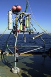
The time-lapse bottom photographs were obtained by means of a Benthos 35-mm camera mounted on a tripod frame that rests on the sea floor
(figure 2 and
figure 3). The camera
(figure 4) was mounted
about 1.5 m above the sea floor and aimed downwards; a strobe
(figure 5) illuminated the
sea floor from one side of the image. The field of view of the camera is 54 degrees,
resulting in an image area measuring approximately 1.5 m x
1 m. A compass and vane (figure 6) mounted in the field of view of the camera show direction
of current flow, scale, and orient the images to north. Instrumentation mounted on the same
tripod frame measured current speed and direction, temperature, light transmission, conductivity,
and pressure every 3.75 minutes. (See
Butman and others, 2002
for a description of these instrument systems.)
The images were taken on Kodak Ektachrome Professional Film (E200, a daylight-balanced 200-speed
color transparency film)
(100 foot roll, about 700 images/roll). The Benthos camera places the images in a
nonstandard format along the long axis of the film. This allows a larger image size
of the sea floor than if the image were placed across the film in a standard 35
mm format. The film is advanced using an O-ring drive;
the loose drive and drive-motor inertia result in the distance between frames varying
slightly with each image.
The camera and strobe were controlled by a timer set to obtain
an image every 4 hours. The time of each photograph differs
from a uniform spacing by a few minutes because of drift in this analog controller. A digital
LED clock, separate from the controller, places the hour,
minute, second, and day on each image. The day counter counts to 31 and then rolls back to 1.
Instrument Deployments
Instrumented tripods are deployed and recovered at Site A three times each year,
typically in February, May-June, and September, as part of the USGS study. This report presents images from
three deployments: deployment 569 beginning in May 1999, deployment 625 beginning
in May 2000, and deployment 665 beginning in October 2001 (569, 625 and 665 are
USGS mooring identification numbers). Each
tripod was located 100-150 m southwest of the
USCG B Buoy (National Ocean Service, 1997) on the
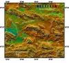
southern flank of a ridge in water about 30 m deep
(figure 7). This location
was selected for the long-term observations because the
USCG Buoy marked the site and provided some protection from human disturbance.
Time-series photographs from other deployments at Site A may be found in other
USGS Data Series Publications.
| ID |
Start/Stop Date |
Latitude (N) |
Longitude (W) |
Water
Depth
(m) |
| 569 |
May 11, 1999 to
Sept. 15, 1999 |
42° 22.68' |
70° 47.09' |
32.9 |
| 625 |
May 13, 2000 to
Sept. 11, 2000 |
42° 22.69' |
70° 47.09' |
29.5 |
| 665 |
Oct. 23, 2001 to
Feb. 6, 2002 |
42° 22.68' |
70° 47.09' |
30.0 |
Movie Creation
Time-lapse movies were created from the individual bottom photographs. Each image
on the 35 mm film was digitized as a .tiff image at a
resolution of 4238 by 2626 pixels by Amaranth Photo Imaging. The
exposure was kept constant for all frames, so that changes in light intensity reflect
changes in water clarity, instrument fouling, or ambient light. The images were reduced to
600 by 372 pixels using PolyView (www.polybytes.com);
this image size was chosen to balance resolution and publication size. The camera controller was set to
obtain an image every 4 hours. However, this controller (separate from the digital
LED clock that placed a time stamp on the images) drifts by
a few minutes over the course of the deployment. For the purposes of the movie, the images
were distributed at an even interval between the start and stop time of the photographic record,
as determined from the LED clock. The camera controller
occasionally missed an image or exposed multiple frames; missed images were filled with blanks
and multiple images deleted. MATLAB software (www.mathworks.com) was used to align the images, make the data plots, and create the .avi movie.
Description of Movie Frames
Each movie frame includes an image of the sea floor at the top and shows oceanographic
data collected at the same time at the bottom. The movie plays at 3 frames/second or 2 seconds/day.
The field of view of the image is approximately 1.5 m wide and
1 m high. The vane on the compass in the images swings with the current and points in the direction of current flow. (Sometimes the vane swivel gets stuck preventing the vane from aligning with the current.) The triangular black arrow on the compass points toward magnetic north (16 degrees west of true north at Site A). The white
arrow in the upper left of the frame points toward true north. The file name of the image is in the
upper left corner of each frame. (This number provides a key to the individual .tif images;
see ‘Images’ in the table below.) The red digits in the lower left corner of the image show time
(in Eastern Standard Time): HR.MM (hour and minute) on the upper line and SS.DD (second and day)
on the second line. The day (DD) counter rolls over every 31 days and thus does not indicate true day of
month for the entire deployment; the correct day of the month is below the data panel. (See below.) The
third line of red digits is a record identifier (NN, the last two digits of the
USGS mooring number).
Below the image to the right is a data panel that shows a plot of current speed (in
cm/s at 1 m above bottom
(mab) (in red);
beam attenuation (in m-1), a measure
of water clarity, at about 2 mab (in blue);
standard deviation of bottom pressure (in mb), a measure of
wave intensity, at about 2 mab (in black); and water temperature (in degrees C), at about 2
mab) (in green) obtained every 3.75 minutes. The
values of current speed, beam attenuation, standard deviation of pressure, and bottom temperature at the time of the photograph are also listed in the data panel. The vertical black line in the center of the data panel is the time of the photograph. The plot shows
4 days of data, 2 before and 2 after the image displayed was obtained. Below the image to the
left is a vector plot showing current speed (length of line)
and direction toward which the current flows (true north is up in this display).
The time below the data panel is the time for each image (in Greenwich Mean Time), computed by evenly spacing the images over the deployment. This evenly-spaced time and frame number are tabulated in an Excel file to facilitate finding a specific image. The best estimate of the time of the image is obtained from the hour and minute recorded by the digital clock on the image (in EST) and the day from the data panel (or from the framelist).
Play Movies and View Images
The movies may be viewed using an image viewer such as QuickTime or Windows Media
Player. Click on Movie in the table below to open the movie, or navigate to the
file on the DVD (in the subdirectory “IMAGES”
in each individual tripod directory) and open with an image viewer. Click on Images
to open thumbnails of individual images; click on an image to view the image, in .tif format, at a
resolution of 600x372 pixels. Each set of images contains several hundred images and may take
a few minutes to load.
| ID | Start Date | Stop Date | View Movie |
View Images |
| 569 |
May 11, 1999 |
Sept. 15, 1999 |
Movie |
Images |
| 625 |
May 13, 2000 |
Sept. 11, 2000 |
Movie |
Images |
| 665 |
Oct. 23, 2001 |
Feb. 6, 2002 |
Movie |
Images |
Highlights of Bottom Processes
The time-lapse movies show changes in the sea floor and bottom water characteristics. A major process
illustrated in these photographs is the resuspension of sediments caused by currents associated with waves.
Increases in beam attenuation (decreased water clarity) usually coincide with periods of increased wave
intensity (caused by storms) and visible cloudiness in the photographs. The sea floor in this region of
Massachusetts Bay is mostly cobbles, pebbles, and coarse sand. However, there are patches of fine-grained
sediment to the west of this site (figure 7),
and a thin veneer of fine sediments is likely to accumulate at the tripod site during times when it is not
stormy. The fine sediments are resuspended by the strong oscillatory currents associated with surface waves.
In some of the events, a pebble or cobble shifts position on the sea floor. Other observations and modeling
suggest that fine sediment resuspended during storms in this region of western Massachusetts Bay is transported
to the southeast toward Cape Cod Bay and offshore into Stellwagen Basin
(Butman and Bothner, 1997). These basins are
long-term depositional sites in the Massachusetts Bay region. Changes in the sea floor when it is not stormy
may be caused by actions of fish or other organisms that do not appear in the 4-hourly images. Note that
objects, such as fish, close to the
camera lens, appear larger than they are in relation to features on the sea bottom.
Oceanographic Data
The time series data of current, temperature, light transmission, beam attenuation, and
pressure shown in the movies obtained at site A are available in
Butman and others (2002).
MATLAB m-files
MATLAB software (www.mathworks.com)
was used to align the images, make the data plots, and create the .avi movie and
thumbnail Web pages. M-files may either be opened within a text viewer or within the
MATLAB editor. To download the m-files click on the links below.
Although these programs have been used by the USGS, no warranty, expressed or implied, is made by the USGS or the United States Government as to the accuracy and functioning of the programs and related program material nor shall the fact of distribution constitute any such warranty, and no responsibility is assumed by the USGS in connection therewith.
Acknowledgments
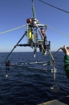
J. Borden and M. Martini prepared the instruments for deployment.
F. Lightsom processed the time-series data. We thank the officers and crew of the
USCG Cutter White Heath and
USCG Cutter Marcus Hannah for deployment and
recovery of instruments at sea. This work was supported by the U.S. Geological Survey Coastal
and Marine Geology Program and by the Massachusetts Water Resources Authority.
References Cited
Butman, Bradford, Alexander, P.S., Bothner, M.H., 2004a, Time-series photographs
of the seafloor in western Massachusetts Bay: June 1997 to June 1998: U.S. Geological Survey
Data Series 87, 1 DVD-ROM.
Butman, Bradford, Alexander, P.S., Bothner, M.H., 2004b, Time-series photographs
of the seafloor in western Massachusetts Bay: June 1998 to May 1999: U.S. Geological Survey
Data Series 96, 1 DVD-ROM.
Butman, Bradford. and Bothner, M.H., 1997, Predicting the long-term fate of sediments and
contaminants in Massachusetts Bay: U.S. Geological Survey Fact Sheet 172-97.
(Also available online at
http://pubs.usgs.gov/fs/fs172-97/.) (Accessed October 15, 2004.)
Butman, Bradford, Bothner, M.H., Lightsom, F.L., Gutierrez, B.T., Alexander, P.S.,
Martini, M.A., and Strahle, W.S., 2002, Long-term observations in western Massachusetts
Bay offshore of Boston, Massachusetts; Data report for 1989 – 2000:
U.S. Geological Survey Digital Data Series DDS-74, 1
DVD-ROM. (Also available online at
http://pubs.usgs.gov/dds/dds74/.)
(Accessed October 15, 2004.)
Butman, Bradford, Hayes, Laura, Danforth, W.W., and Valentine, P.C., 2003, Backscatter
intensity, shaded relief, and sea floor topography of Quadrangle 2 in western Massachusetts Bay offshore
of Boston, Massachusetts: U.S. Geological Survey Geologic Investigations Series
Map I-2732-C, scale 1:25,000. (Also available online at
http://pubs.usgs.gov/imap/i-2732c/.)
(Accessed October 15, 2004.)
National Ocean Service, 1997, Massachusetts Bay: National Oceanic and Atmospheric Administration,
National Ocean Service, Chart 13267, scale 1:80,000.
U.S. Geological Survey, 2004, Boston sewage outfall: The fate of sediments and
contaminants in Massachusetts Bay: U.S. Geological Survey Web site at
http://woodshole.er.usgs.gov/project-pages/bostonharbor/. (Accessed October 15, 2004.)

 To view files in PDF format, download free copy of Adobe Reader. To view files in PDF format, download free copy of Adobe Reader.
|