Introduction This report presents time-series photographs of the sea floor obtained from an instrumented tripod deployed at LT-A in western Massachusetts Bay (42° 22.6' N., 70° 47.0' W., 33 m water depth, fig. 1) from December 1989 through June 1993. Time-series photographs and oceanographic observations were initiated at LT-A in December 1989 and continued through February 2006. This is one of a series of reports that present these photographs in digital form (Butman and others 2004a, b, and c; table 1). The objective of these reports is to enable easy and rapid viewing of the photographs and to provide a medium-resolution digital archive. The photographs, obtained every 4 or every 6 hours, are presented as a movie (in .avi format) and as individual photographs (in .png format). The photographs provide time-series observations of changes of the sea floor, near-bottom water turbidity, and life on the sea floor. The time-series photographs taken at LT-A were collected as part of a U.S. Geological Survey (USGS) study to understand the transport and fate of sediments and associated contaminants in Massachusetts and Cape Cod Bay (Bothner and Butman, 2007). This long-term study was carried out by the USGS in partnership with the Massachusetts Water Resources Authority (MWRA) (http://www.mwra.state.ma.us/) and with logistical support from the U.S. Coast Guard (USCG). Long-term oceanographic observations help to identify the processes causing bottom sediment resuspension and transport and provide data for developing and testing numerical models. The observations document seasonal and interannual changes in currents, hydrography, and suspended-matter concentration, and the importance of infrequent catastrophic events, such as major storms, in sediment resuspension and transport. LT-A is approximately 1 km south of the ocean outfall that began discharging treated sewage effluent from the Boston metropolitan area into Massachusetts Bay in September 2000. See Butman and others (2004d) for a description of the oceanographic measurements at LT-A and Butman and others (2007c) for discussion of sediment transport in Massachusetts Bay. Instrumentation The time-lapse bottom photographs were obtained by means of a Benthos 35-mm camera mounted on a tripod frame that rests on the sea floor (figs. 2 and 3). The camera (fig. 4) was mounted about 1.5 m above the sea floor and aimed downwards; a strobe (fig. 5) illuminated the sea floor from one side of the photograph. The field of view of the camera is 54 degrees, resulting in a photograph area on the sea floor measuring approximately 1.5 m x 1 m. A compass and vane (fig. 6) mounted in the field of view of the camera show the instantaneous direction of current flow, and the scale and orientation of the photographs. The photographs were taken on Kodak 35-mm Ektachrome Professional Film (E200, a daylight-balanced 200-speed color transparency film) (100-ft roll, about 700 photographs/roll). The Benthos camera places the photographs in a nonstandard format along the long axis of the film. This allows a photograph of the sea floor larger than what would be possible if the photograph were placed across the film in a standard 35-mm format. The film is advanced using an O-ring drive; the loose drive and drive-motor inertia result in the distance between frames varying slightly with each photograph. The unevenly spaced photographs required alignment to view them as a time-series movie without jitter. The camera and strobe were controlled by a timer set to obtain a photograph every 4 or 6 hours, depending on the deployment. The time of each photograph differs from a uniform spacing by a few minutes because of drift in this analog controller. A digital light emitting diode (LED) clock, separate from the controller, places the hour, minute, second, and day on each photograph. The day counter on the LED clock counts to 31 and then resets back to 1. The time on the LED typically differed from true time by a few minutes at the end of the deployment and thus is assumed to provide a reasonably accurate time for each photograph. Instrumentation mounted on the same tripod frame measured current speed and direction, temperature, light transmission, conductivity, and pressure every 3.75 minutes. Butman and others (2004d) describe these instrument systems. Light transmission is a measure of water clarity and was converted to beam attenuation (attenuation = - 4ln(percent transmission over 0.25 m)). Current was sampled, typically at 2 Hz, and vector-averaged to provide a mean current every 3.75 minutes. Pressure was also sampled at 2 Hz; the standard deviation of pressure (called PSDEV) was computed every 3.75 minutes as a measure of wave-induced fluctuations at the sea floor. Plots of these data are included in the .avi movies. Instrument Deployments During the USGS study, instrumented tripods were deployed and recovered at LT-A three times each year, typically in February, May or June, and September. This report presents photographs obtained during nine deployments that took place during the period December 1989 through June 1993; the deployments are identified by a 3-digit USGS mooring number that is assigned sequentially to all instrument deployments (table 2). Each tripod was located 100-150 m southwest of the USCG B Buoy (National Ocean Service, 1997) on the southern flank of a ridge in water about 33 m deep (fig. 7). This location was selected for long-term observations because a USCG buoy marked the site and provided some protection from other marine activities. Time-series photographs from subsequent deployments at LT-A are presented in other USGS Data Series publications (table 1). Table 2. USGS mooring number, date and location of time-series photographs contained in this Data Series report. Mooring Number Start Date Stop Date Latitude (N) Longitude (W) Water Depth Depth (m) 338 December 5, 1989 March 28, 1990 42° 23.65' N 70° 47.27' W 29 347 July 10, 1990 October 23, 1990 42° 22.66' N 70° 46.97' W 34 358 October 24, 1990 February 12, 1991 42° 22.62' N 70° 47.10' W 30 374 February 12, 1991 June 11, 1991 42° 22.62' N 70° 47.12' W 30 383 June 11, 1991 October 15, 1991 42° 22.63' N 70° 47.07' W 30 389 October 16, 1991 October 30 1991 42° 22.63' N 70° 47.11' W 30 400 June 2, 1992 October 20, 1992 42° 22.63' N 70° 47.07' W 30 407 October 20, 1992 February 18, 1993 42° 22.62' N 70° 47.07' W 30 413 February 25, 1993 June 15, 1993 42° 22.47' N 70° 47.12' W 32 Digitizing the Films Each photograph on the 35-mm film was digitized as a .tiff at a resolution of 1920 by 1080 pixels at the Woods Hole Oceanographic Institution (WHOI) using a special film transport mechanism and aligned using Combustion 4.0 (http://dv411.com/combustion4.html) and Shake 5.0 (http://www.apple.com/shake) software. The photographs were reduced to 600 by 337 pixels using PolyView (www.polybytes.com) and compressed to 256-color .png images using IrfanView (http://www.irfanview.com), reducing the photograph size by about a factor of 6. This photograph size and compression provide reasonable resolution and manageable size for this publication. The full resolution digital photographs and the original 35-mm films are archived at the USGS Woods Hole Science Center. Creating the Time-Lapse Movies Time-lapse movies were created from the digitized photographs using MATLAB software (www.mathworks.com). The photographs collected at approximately 4-hour intervals (deployments 338 through 383) or 6-hour intervals (deployments 389 through 413), within a few minutes, were distributed at an even interval between the start and stop time of the photographic record, as determined from the LED clock. During the deployment, the camera controller occasionally malfunctioned; to provide an equally spaced time-series, missed photographs were filled with blanks and multiple photographs were deleted. The data plots shown with the photographs also were made with MATLAB. The movies were compressed with the Microsoft Video 1 codec using VideoMach (http://www.gromada.com/). This reduced the .avi file size by a factor of about 6. Viewing Movies and Photographs The movies may be viewed using a movie player such as QuickTime, Imagen, or Windows Media Player. Click on Movie in Table 3 to open the movie, or navigate to the .avi file on the DVD (located in directories labeled TRIPODNNN, where NNN is the mooring number) and open with a movie player. Click on Photographs in Table 3 to open a page of thumbnails of individual photographs; click on a thumbnail to view the photograph, in .png format, at a resolution of 600x337 pixels. Table 3. Click on Movie to open the movie with a movie player such as Imagen, Quicktime or Windows Media Player. Or right click on Movie to download the .avi file to your hard drive. Some movie players allow adjustment of play speed, scanning of the movie by dragging a location slider with a mouse, and/or control of the movie one frame at a time forward or backward. Click on Photographs to open a page of thumbnails of the individual photographs; click on a thumbnail on the thumbnail page to view a larger-format photograph (in .png format). Click on Comments for a list of features and events of note for each set of time-series photographs. Mooring Number Start Date Stop Date Movie Photographs Comments 338 December 5, 1989 March 28, 1990 Movie Photographs Comments 347 July 10, 1990 October 23, 1990 Movie Photographs Comments 358 October 24, 1990 February 12, 1991 Movie Photographs Comments 374 February 12, 1991 June 11, 1991 Movie Photographs Comments 383 June 11, 1991 October 15, 1991 Movie Photographs Comments 389 October 16, 1991 October 30, 1991 Movie Photographs Comments 400 June 2, 1992 October 20, 1992 Movie Photographs Comments 407 October 20, 1992 February 18, 1993 Movie Photographs Comments 413 February 25, 1993 June 15, 1993 Movie Photographs Comments Description of Movie Frames Each movie frame includes a photograph of the sea floor at the top of the frame and shows oceanographic data collected at the same time at the bottom of the frame. The movie plays at 3 frames/second (1.3 seconds/day for photographs every 6 hours, or 2 seconds/day for photographs every 4 hours). The field of view of the photograph is approximately 1.5 m wide and 1 m high. The vane on the compass in the photographs swings with the current and points in the direction of current flow. The triangular black arrow on the compass points toward magnetic north (16 degrees west of true north at LT-A). The white arrow in the upper left of the frame points toward true north. The file name of the photograph is in the upper left corner of each frame. This number provides a key to the individual photograph; see 'Photographs' in table 3. The red digits in the lower left corner of the photograph show time (in Eastern Standard Time): HR.MM (hour and minute) on the upper line and SS.DD (second and day) on the second line. The day (DD) counter rolls over every 31 days and thus does not indicate true day of month for the entire deployment; the correct day of the month is below the data panel (see below). The third line of red digits is a record identifier (N.N., the last two digits of the USGS mooring number). Below the photograph to the right is a data panel that shows a plot of current speed (in cm/s at 1 m above bottom (mab) (in red); beam attenuation (in m-1), a measure of water clarity, at about 2 mab (in blue); standard deviation of bottom pressure (PSDEV) in mb), a measure of wave intensity, at about 2 mab (in black); and water temperature (in degrees C), at about 2 mab) (in green) obtained every 3.75 minutes. The values of current speed, beam attenuation, standard deviation of pressure, and bottom temperature at the approximated time of the photograph (by evenly spacing the photographs over the deployment period) are also listed in the data panel. The vertical black line in the center of the data panel is the time of the photograph. The plot shows 4 days of data, 2 days before and 2 days after the photograph displayed was obtained. Below the photograph to the left is a vector plot showing current speed (length of line) and direction toward which the current flows (true north is up in this display). The time below the data panel is the time for each photograph (in Greenwich Mean Time), computed by evenly spacing the photographs over the deployment. This evenly-spaced time and frame number are tabulated in an Excel file to facilitate finding a specific photograph. The best estimate of the time of the photograph is obtained from the hour and minute recorded by the digital clock on the photograph (in EST), and the day from the data panel (or from the framelist.xls). Table 4. Link to tables in Excel format that lists frame number and frame date and time for each deployment. [GMT, Greenwich Mean Time]. Mooring Number Table of frame date and time (GMT) 338 framelist338.xls 347 framelist347.xls 358 framelist358.xls 374 framelist374.xls 383 framelist383.xls 389 framelist389.xls 400 framelist400.xls 407 framelist407.xls 413 framelist413.xls Highlights of Time-Series Photographs The sea floor in the area of tripod deployments in western Massachusetts Bay is typically covered by gravel and cobbles. Although deployed within about 100 m of each other (fig. 7), the sea floor under each tripod is unique. The placement of the camera, strobe, and compass on the tripod frame differs slightly from deployment to deployment, and thus each set of time-series photographs have different lighting and field of view. Each set of time-series photographs presents a unique view of approximately a 1-m2 area of the sea floor and show changes in the sea floor, near-bottom water turbidity, and plants and animals. Some features and events for each set of time-series photographs are provided in the Comments Section. Animals occasionally appear in the photographs, sometimes remaining in the field of view for more than one photograph. Identification of some of the animals and plants in the photographs is given in table 5. Note that objects, such as fish, close to the camera lens, appear larger than they are in relation to features on the bottom. Some of the deployments have unique characteristics that are a result of the unattended operation of the equipment on the ocean bottom. In some deployments, the lighting decreases with time due to failure of the strobe battery, biological fouling on the strobe bulb or reflector that interferes with the light reaching the sea floor, or failure caused by corrosion. The oceanographic sensors or recording electronic equipment do not always function properly for the entire 4-month deployment, resulting in loss of data. In other deployments, the tripod frame may be tipped on its side ending the photograph sequence or continuing the sequence, but with the camera no longer focused on the sea floor. A major process illustrated in these photographs is the resuspension of sediments caused by oscillatory currents associated with surface waves. Increases in beam attenuation (indicating decreased water clarity) usually coincide with periods of increased wave intensity (caused by storms) and visible turbidity in the photographs. The sea floor in this region of Massachusetts Bay is mostly covered by cobbles, pebbles, and coarse sand; however, there are patches of fine-grained sediment to the west of this site (fig. 7), and a thin veneer of fine sediments is likely to accumulate at the tripod site during periods of low waves. These fine sediments are resuspended by the oscillatory currents associated with surface waves. In some of the storms, a pebble or cobble shifts position on the sea floor. Other observations and modeling suggest that fine sediment resuspended during storms in this part of western Massachusetts Bay is transported to the southeast toward Cape Cod Bay and offshore into Stellwagen Basin (fig. 1; Butman and others, 2007c). These areas are long-term depositional sites in the Massachusetts Bay region. Changes in the sea floor during non-storm periods may be caused by actions of fish or other organisms that may not appear in the photographs due to the 4- or 6-hour spaced time intervals. Oceanographic Data The time-series data of current, temperature, light transmission, beam attenuation, and pressure shown in the time-lapse movie of the photographs obtained at LT-A are available in Butman and others (2004d). They are archived by mooring number. MATLAB Routines MATLAB software (www.mathworks.com) was used to make the data plots and create the .avi movie and thumbnail Web pages. M-files may either be opened within a text viewer or within the MATLAB editor. To download the m-files, click on the links below.       adjust_image (aligns photographs/creates movie)       find_edges.m (user selects photograph edges)       create_thumbnail_page.m (creates the thumbnail pages) Acknowledgments W. Strahle and M. Martini prepared the instruments for deployment. F. Lightsom processed the time-series data. We thank the officers and crew of the USCG Cutter White Heath for deployment and recovery of instruments at sea. We thank Barbara Hecker and Ken Keay for assistance with the animal identifications. This work was supported by the U.S. Geological Survey Coastal and Marine Geology Program and by the Massachusetts Water Resources Authority. Donna Newman prepared this document in HTML. References Cited Bothner, M.A and Butman, Bradford, eds., 2007, Processes influencing the transport and fate of contaminated sediments in the coastal ocean - Boston Harbor and Massachusetts Bay: U.S. Geological Survey Circular 1302, 87 p. Butman, Bradford, Alexander, P.S., Bothner, M.H., 2004a, Time-series photographs of the sea floor in western Massachusetts Bay - June 1997 to June 1998: U.S. Geological Survey Data Series 87, DVD-ROM. Also online at http://pubs.usgs.gov/ds/2004/87/ Butman, Bradford, Alexander, P.S., Bothner, M.H., 2004b, Time-series photographs of the sea floor in western Massachusetts Bay - June 1998 to May 1999: U.S. Geological Survey Data Series 96, DVD-ROM. Also online at http://pubs.usgs.gov/ds/2004/96/ Butman, Bradford, Alexander, P.S., Bothner, M.H., 2004c, Time-series photographs of the sea floor in western Massachusetts Bay - May 1999 to September 1999; May 2000 to September 2000; and October 2001 to February 2002: U.S. Geological Survey Data Series 97, DVD-ROM. Also online at http://pubs.usgs.gov/ds/2004/97/ Butman, Bradford, Bothner, M.H., Alexander, P.S., Lightsom, F.L., Martini, M.A., Gutierrez, B.T., and Strahle, W.S., 2004d, Long-term observations in western Massachusetts Bay offshore of Boston, Massachusetts; Data report for 1989 - 2000: U.S. Geological Survey Digital Data Series DDS-74, Version 2.0, DVD-ROM. Also online at http://pubs.usgs.gov/dds/dds74/ Butman, Bradford, Dalyander, P.S., Bothner, M.H., Lange, W.H., 2007a, Time-series photographs of the sea floor in western Massachusetts Bay, Version 1, 1989 - 1993: U.S. Geological Survey Data Series 265, Version 1.0, DVD-ROM. Also online at http://pubs.usgs.gov/ds/2007/265/ Butman, Bradford, Hayes, Laura, Danforth, W.W., and Valentine, P.C., 2003, Backscatter intensity, shaded relief, and sea floor topography of Quadrangle 2 in western Massachusetts Bay offshore of Boston, Massachusetts: U.S. Geological Survey Geologic Investigations Series Map I-2732-C, scale 1:25,000. Also online at http://pubs.usgs.gov/imap/i-2732c/ Butman, Bradford, Valentine, P.C., Middleton, T.J., and Danforth, W.W., 2007b, A GIS library of multibeam data for Massachusetts Bay and the Stellwagen Bank National Marine Sanctuary, offshore of Boston, Massachusetts. U.S. Geological Survey Data Series 99, Version 1.0, 1 DVD-ROM. Also online at http://pubs.usgs.gov/ds/99/ Butman, Bradford, Warner, J.C., Bothner, M.H. and Dalyander, P.S., 2007c, Predicting the transport and fate of sediments caused by northeast storms, Section 6 in Bothner, M.A and Butman, Bradford, eds., 2007, Processes influencing the transport and fate of contaminated sediments in the coastal ocean-Boston Harbor and Massachusetts Bay: U.S. Geological Survey Circular 1302. National Ocean Service, 1997, Massachusetts Bay: National Oceanic and Atmospheric Administration, National Ocean Service, Chart 13267, scale 1:80,000.

Click on thumbnail below for figure in PDF format. 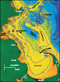Figure 1. Location map. 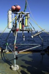Figure 2. Tripod system. 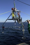Figure 3. Tripod system. 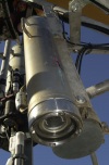Figure 4. Camera. 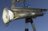Figure 5. Strobe. 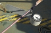Figure 6. Compass. 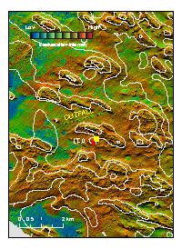Figure 7. Location map. Table 1. Publications. (HTML) 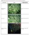Table 5. Animal identifications. (HTML)