USGS PCMSC

Imaging The M7.9 Denali Fault Earthquake 2002 Rupture At The Delta River
Using SASW, LIDAR, and RADAR

Index Back to Home Page About These Web Pages Summary LIDAR & Radar SASW Method and Results Study Area Abstract

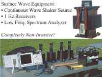
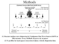
Spectral Analysis of Surface Waves: Method and Results

Click on image to view larger version (42KB, 31KB)
SASW equipment. Diagram of SASW array.
Photo of D9N dozer. To reach the bedrock surface beneath the Delta River on either side of the Denali Fault, we need to use a large energy source. Alyeska Pipeline Services Corp. provided a Caterpillar D9N dozer to produce low frequency, deep sounding surface waves for the SASW tests. For the higher frequency data we used a continuous harmonic-sine source to characterize the stiffness of the upper portion of the soil column.

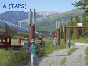
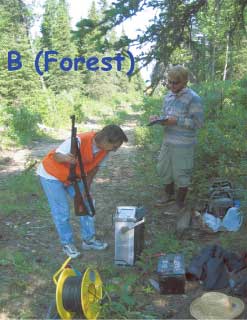
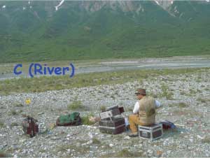
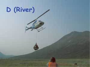
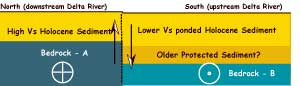
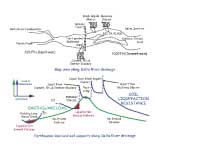
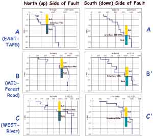
On the Denali fault, ~15% of the surface expression of the 2002 right-lateral oblique rupture was up to the north at the Delta River. We sought to estimate the depth of bedrock on either side of the fault and total relative uplift using Spectral Analysis of Surface Waves. On the Delta River the vertical uplift was between 60-80cm up to the north during the 2002 event.

Photo of cable and seismometer deployment at the TAPS. Recording waveforms on a spectral analyzer along the forest road.
SASW testing on the Delta River. Helicopter dropping SASW equipment at Delta River.
Field Operations: We deployed seismometers at sides on the north and south side of the fault at 3 transect lines. Photographs (A) cable and seismometer deployment at the TAPS; (B) recording waveforms on a spectral analyzer along the forest road...bear country; (C) SASW testing on the Delta River; (D) deployment on the west side of the Delta River required helicopter carries of equipment.

Simplified diagram.

Simplified interpretation of SASW results: Delta River

Tectonic uplift, sediment ponding, and their effects on liquefaction potentialConceptual diagram of the intersection of earthquake load and coil liquefaction resistance capacity.
Click on image to view larger version (19KB, 35KB)
Producing a shear wave velocity profile from the surface wave data involves (1) field collection of cross-power spectra and frequency response data; (2) computing a dispersion curve for Rayleigh waves; and (3) inverting a theoretical shear wave velocity structure whose dispersion curve shape best fits (Minimum RMS deviation) the field dispersion curve. Step (1) involves placement of seismometers at distance from a surface wave source (CAT D9N). From the cross-power spectra and seismometer array geometry we can compute the dispersion curve (2) in the field. We use three independent inversion algorithms to estimate the body wave structure of the ground. The inversion process and its results are non-unique.
SASW results a 3 sites.(View at 50KB) SASW Results: Holocene sediment fill on the north side of the fault is to ~90m in all three transects. On the south side, the sediment depth varies between 145-185 meters, and a higher velocity (older) sediment unit is present and possibly protected by the fault scarp. We estimate that there is between 55-95 meters of relative vertical offset, up to the north, since the entire valley was glacially scoured to bedrock. Fault offset ponds sediment on the south side of the fault. Accretion in this quieter depositional environment results in higher liquefaction potential (Kayen et al. Earthquake Spectra 20(3) 639-667).

Poster Home Page | Abstract | Study Area | SASW Method & Results | LIDAR & Radar | Summary | About These Web Pages
Geotech Home Page

geotech/denlidaposter/sasw.html
contact: Robert Kayen
last modified 2018