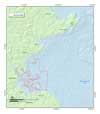
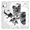
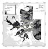
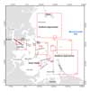
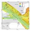
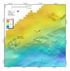
Figure 1.1. Map showing the location of the Boston Harbor and Approaches area, offshore of Massachusetts. The geophysical data used in this report are from four NOAA hydrographic surveys (H10990, H10991, H10992, and H0994) carried out in 2000 and 2001 (outlined in red).
|
|
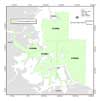
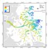
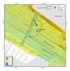
Figure 1.2. Map showing the location of the NOAA hydrographic surveys H10990, H10991, H10992, and H0994 that collected the bathymetry and sidescan-sonar data used to map the sea floor of Boston Harbor and Approaches.
|
|
Figure 3.1. Photograph of the NOAA Ship Whiting. The Whiting, 163’ long and equipped with two launches to carry out hydrographic surveys, was decommissioned by NOAA in 2003.
|
|
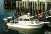
Figure 3.2. Photograph of the USGS research vessel Rafael. The Rafael is 25’ long and used by USGS to conduct geophysical surveys in coastal areas.
|
|
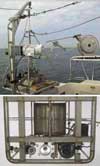
Figure 3.3. TOP: Photograph of Mini SEABOSS and winch on the deck of the RV Rafael. On the Rafael, the SEABOSS sits on a frame mounted outboard of the vessel. The conducting cable that carries power and the video signal is stored on the cable spool. BOTTOM: Components of Mini SEABOSS viewed from below: A) forward video camera; B) downward video camera; C) video light; D) digital still camera and housing; E) strobe light; F) parallel laser for scale; G, laser for ranging; H) junction block; I) van Veen grab sampler; and J) multi-conducting cable.
|
|
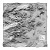
Figure 3.4. Map showing mosaic of sidescan-sonar data of the survey area Boston Harbor and Approaches, Massachusetts. Backscatter intensity, as recorded with sidescan-sonar, is an acoustic measure of the hardness and roughness of the sea floor. In general, higher values (light tones) represent rock, gravel and coarse sand. Lower values (dark tones) generally represent fine sand and muddy sediment. See map sheet 3 for data at a scale of 1:25,000.
|
|
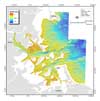
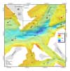
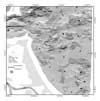
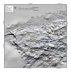
Figure 3.5. Shaded-relief bathymetric map, colored by water depth, of Boston Harbor and Approaches, Massachusetts based on the multibeam sonar data (gridded at 2 m). See map sheet 2 for date at a scale of 1:25,000.
|
|
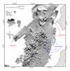
Figure 3.6. Shaded-relief bathymetric map, colored by water depth, of Boston Harbor and Approaches, Massachusetts, based on the combined multibeam and single-beam sonar bathymetric data (gridded at 30 m). See map sheet 1 for data at a scale of 1:25,000.
|
|
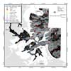
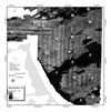
Figure 3.7. Map showing location of bottom samples on a map of acoustic backscatter intensity from sidescan-sonar. Each numbered circle indicates a station where photographs, video, and/or samples were collected. See map sheet 5 for figure at a scale of 1:60,000.
|
|
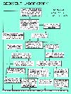
Figure 3.8. Flow diagram showing steps in laboratory analysis of sediment samples carried out at the USGS sediment laboratory at the Woods Hole Science Center (Poppe and Polloni, 2000).
|
|
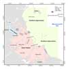
Figure 4.1. Map showing Boston Inner Harbor, Outer Harbor, and the Northern and Southern Approaches.
|
|
Figure 4.2. Map of Boston Harbor and Approaches showing locations of Figures 4.4 – 4.20 that illustrate selected features and characteristics of the sea floor.
|
|
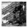
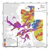
Figure 4.3. Texture of surficial sediments, based on Shepard classification, superimposed on gray-scale sidescan-sonar mosaic of Boston Harbor and Approaches. Dark blue dots indicate sites where no sample was collected and photographs show the sea floor is bedrock or covered with boulders, cobble or shells. Low backscatter intensity corresponds to areas of fine-grained sediments (silt and clay, Inner Harbor) or sandy sediments (Approaches). High backscatter intensity corresponds to areas of gravel, boulders, or outcropping bedrock (areas that could not be sampled with the grab sampler). See Appendix 2 for sediment texture and Appendix 3 for bottom photographs. See map sheet 5 for figure at a scale of 1:60,000.
|
|
Figure 4.4. Shaded relief bathymetry, colored by water depth, of eastern portion of Boston Inner Harbor showing dredged main shipping channel, Ted Williams Tunnel, circular dredged areas south of Logan Airport, cable crossing, and linear scour marks. See Figure 4.2 for map location. Red dots show location of bottom photographs (see Appendix 3 to view all photographs at these locations); yellow dot is location of bottom sediment sample (Appendix 2); number is station identifier.
|
|
Figure 4.5. Shaded relief bathymetry, colored by water depth, showing the Ted Williams Tunnel as it crosses Boston Inner Harbor from south Boston to Logan Airport (see fig. 4.2 for map location). The tunnel is marked by a depression about 50 m wide that is a few m deeper than the navigation channel; on the northern side of the channel, the tunnel depression has a central high and channels about 2-4 m deeper along the western and eastern edges. Red dots show location of bottom photographs (see Appendix 3 to view all photographs at these locations); yellow dot is location of bottom sediment sample (Appendix 2); number is station identifier.
|
|
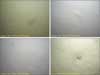
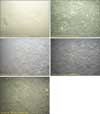
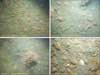
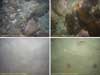
Figure 4.6. Photographs of the sea floor in Boston Inner Harbor stations 104, 103, 105, 101 showing a muddy sea floor. See Figure 4.3 for station locations. See Appendix 3 for more photographs at these stations. The field of view of each image is approximately 50 cm wide.
|
|
Figure 4.7. Shaded-relief bathymetry, colored by water depth, of the depression south of Deer Island where the deepest water in Boston Harbor occurs (about 28 m deep). See Figure 4.2 for map location. Red dots show location of bottom photographs (see Appendix 3 to view all photographs at these locations); yellow dot is location of bottom sediment sample (Appendix 2); number is station identifier.
|
|
Figure 4.8. Shaded-relief bathymetry, colored by water depth, showing sand waves along the northern side of the navigation channel south of Deer Island (see fig. 4.2 for map location). The sand waves are less than a meter high and have wavelengths of about 10 m. Red dots show location of bottom photographs (see Appendix 3 to view all photographs at these locations); yellow dot is location of bottom sediment sample (Appendix 2); number is station identifier.
|
|
Figure 4.9. Photographs of the sea floor along the navigation channel, showing the transition for fine-grained mud in the inner harbor to a gravel pavement in the outer harbor (stations 101, 70, 53, 54, and 44). See Figure 4.3 for station locations. See Appendix 3 for more photographs at these stations. The field of view of each image is approximately 50 cm wide.
|
|
Figure 4.10a. Shaded-relief bathymetry showing disposal of dredged material in the topographic low north of Hull. See Figure 4.2 for map location. See Appendix 3 for photographs at Station 62.
|
|
Figure 4.10b. Shaded-relief bathymetry, colored by water depth, showing disposal of dredged material in the topographic low north of Peddocks Island. See Figure 4.2 for map location.
|
|
Figure 4.11. Photographs of the sea floor in areas of high backscatter intensity north, east and south of Peddocks Island (stations 62, 58, 65, and 67). See Figure A3.1 for station locations. See Appendix 3 for additional photographs at these stations. The field of view of each image is approximately 50 cm wide.
|
|
Figure 4.12. Photographs of the sea floor in areas of low backscatter intensity south of Long Island and southeast of Peddocks Island (stations 63 and 61). See Figure A3.1 for station locations and Figure 4.3 for sediment texture. See Appendix 3 for additional photographs at these stations. The field of view of each image is approximately 50 cm wide.
|
|
Figure 4.13. Photographs of the sea floor in the south Channel (station 50) and in a small area of low backscatter intensity southeast of Deer Island (station 45). See Figure A3.1 for station locations locations. See Appendix 3 for additional photographs at these stations. The field of view of each image is approximately 50 cm wide.
|
|
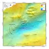
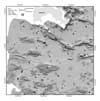
Figure 4.14a. Shaded-relied bathymetric map of the Approaches to Boston Harbor, north of the Harbor Islands and south of Nahant, including Broad Sound (see fig. 4.2 for map location). The darker patches indicate the areas where multibeam bathymetry was collected and data gridded at 2 m; the rest of the area was mapped by single-beam sonar and gridded at 30 m. The sea floor in this region is characterized by elevated rough areas, some of which are hypothesized to be drumlins reworked by rising sea level. See Figure 4.15 for selected photographs at stations 72, 73, and 84. See Figure 4.14b for companion sidescan-sonar image.
|
|
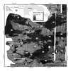
Figure 4.14b. Backscatter intensity from sidescan-sonar of the Approaches to Boston Harbor, north of the Harbor Islands and south of Nahant, including Broad Sound (see fig. 4.2 for map location). The sea floor in this region is characterized by elevated rough areas, some of which are hypothesized to be drumlins reworked by rising sea level. Red dots show location of bottom photographs (see Appendix 3 to view all photographs at these locations); yellow dot is location of bottom sediment sample (Appendix 2); number is station identifier. See Figure 4.14a for companion shaded-relief map.
|
|
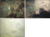
Figure 4.15. Photographs of the sea floor in areas of elevated topography, rough sea floor, and high backscatter intensity (stations 73 and 84, fig. 4.14) in Broad Sound. The boulders are covered with a pink calcareous algae. The sea floor between these features is sand (station 72). See Figure 4.14b for station locations. See Appendix 3 for additional photographs at these stations. The field of view of each image is approximately 50 cm wide.
|
|
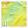
Figure 4.16a. Shaded-relief bathymetric map showing outcropping ledges east of the Brewster Islands (see fig. 4.2 for map location). The darker patches indicate the areas where multibeam bathymetry was collected and the data gridded at 2 m; the rest of the area was mapped by single-beam sonar and the data gridded at 30 m. These ENE-WSW-trending features exhibit the largest topographic variability in the study area. See Figure 4.16b for companion sidescan sonar image.
|
|
Figure 4.16b. Backscatter intensity from sidescan-sonar showing outcropping ledges east of the Brewster Islands (see fig. 4.2 for map location). These ENE-WSW-trending features exhibit the largest topographic variability in the study area and are characterized by moderate backscatter intensity. Red dots show location of bottom photographs (see Appendix 3 to view all photographs at these locations); yellow dot is location of bottom sediment sample (Appendix 2); number is station identifier. See Figure 4.16a for companion shaded-relief map.
|
|
Figure 4.17a. Shaded-relief bathymetric map, colored by water depth, showing elevated areas and sand ribbon, east of Nantasket Beach (see fig. 4.2 for map location). The darker patches indicate the areas where multibeam bathymetry was collected and the data gridded at 2 m; the rest of the area was mapped by single-beam sonar and the data gridded at 30 m. See Figure 4.17b for companion sidescan-sonar image. See Figure 4.18 for selected photographs at stations 5, 6, 8, and 10.
|
|
Figure 4.17b. Backscatter intensity from sidescan-sonar of area east of Nantasket Beach (see fig. 4.2 for location). The elevated areas are characterized by high backscatter intensity and the sand ribbon by low backscatter intensity. Red dots show location of bottom photographs (see Appendix 3 to view all photographs at these locations); yellow dot is location of bottom sediment sample (Appendix 2); number is station identifier. See Figure 4.17a for companion shaded-relief map.
|
|
Figure 4.18. Photographs of the sea floor in areas of elevated topography, rough sea floor, and high backscatter intensity (stations 8 and 10, 11.0 and 11.5 m water depth respectively) east of Nantasket. The pink on the boulders is calcareous algae. The sea floor between these features is sand (stations 5, 6, 13.4 and 16.0 m water depth respectively). See Figure 4.17b for station locations. See Appendix 3 for additional photographs at these stations. The field of view of each image is approximately 50 cm wide.
|
|
Figure 4.19. Shaded-relief bathymetric map showing numerous individual targets 4-6 m on a side and less than a meter high that are interpreted to be individual boulders. Similar targets are observed in the 2-m multibeam bathymetry in nearly all of the areas with a rough sea floor. See Figure 4.2 for map location.
|
|
Figure 4.20. Shaded-relief bathymetry bathymetric map of the area west of Great Brewster and Calf Island showing barge wrecks and mounds of dredged material on the sea floor. See Figure 4.2 for map location.
|
|
Figure 4.21. Physiographic units of the sea floor of Boston Harbor and Approaches, based on bottom roughness, backscatter intensity, and sediment texture.
|
|
Figure 4.22. Sidescan sonar mosaic (A) assembled in the field during the hydrographic surveys and (B) the mosaic assembled from reprocessed sidescan-sonar data. The mosaics are qualitatively similar, but the reprocessed mosaic has more uniform intensity and improved resolution.
|
|
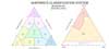
Figure A2.1. Texture of surficial sediment collected in grab samples shown on a ternary diagram. The stations are keyed to the map units (see fig. 4.21). Texture of the rough sea-floor zones is not represented, as samples could not be collected in areas of boulders or gravel pavement.
|
|
Figure A3.1. Map showing bottom sample locations and bottom photo locations overlain on the sidescan-sonar imagery. Photographs and video were obtained at all sites. Samples could not be collected at sites where the bottom was cobble or rocky (yellow dots).
|
|


 Back to Table of Contents
 Forward to Next Section