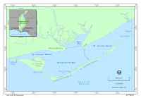
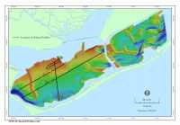
 | Figure 1. Map of Apalachicola Bay identifying regional geographic locations, physiographic features, and water bodies. Inset illustrates the location of the bay within the southeastern United States. |
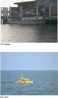 | Figure 2. Photographs of the survey platforms used in this study: R/V Rafael and Autonomous Surface Vehicle IRIS. |
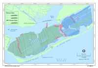 | Figure 3. Map showing geophysical track lines occupied by R/V Rafael and Autonomous Surface Vehicle IRIS during survey cruises in 2005 and 2006. |
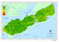
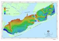 | Figure 4. Bathymetric map of the Apalachicola Bay estuary. See also Mapsheet 1. |
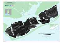
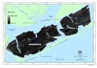 | Figure 5. Sidescan-sonar image of the Apalachicola Bay estuary. See also Mapsheet 2. |
 | Figure 6. Map showing the names of bay-floor and geographic features within the Apalachicola Bay study area. Locations of sediment samples collected by NOAA Coastal Services Center (NOAA, 1999) that were used to verify the sidescan-sonar interpretation are shown. |
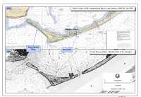 | Figure 7. 2000 NOAA chart # 11402 (top panel) and 1860 NOAA chart # 485 (bottom panel) showing the location of New Inlet, a former tidal inlet near Higgins Shoal that presently is sealed (NOAA, 1860; 2000). |
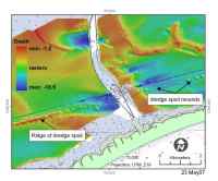 | Figure 8. Bathymetric map of the Intracoastal Waterway near the Bryant Patton Bridge showing dredged material south of its channel. |
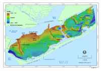
 | Figure 9. Map showing the slope of the bay floor. The steepest slopes are found along the flanks of the Intracoastal Waterway, along the margins of the bay, and on the western sides of linear bars (eg. St. Vincent's Bar and Porter's Bar). |
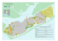
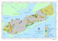 | Figure 10. Map showing the distribution of eleven sedimentary facies identified on the floor of Apalachicola Bay superimposed on the shaded-relief image of the bathymetry. |
 | Figure 11. Interpreted seismic profile showing the stratigraphic intervals underlying Apalachicola Bay. The deepest horizon imaged is the floor of a Pleistocene river valley. This valley was filled during the Early and Middle Holocene by estuarine deposits. During the Late Holocene, a delta system advanced into the bay. Presently mud derived form the Apalachicola River blankets large parts of these older stratigraphic intervals. Vertical scales for the seismic profile are provided in milliseconds (two-way travel time) and approximate depth in meters (assuming a seismic velocity of 1500 m/s). The location of profile 11 is identified on seismic profile A of figure 12 and also in figure 13. |
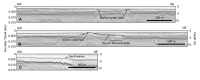
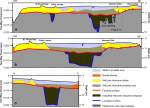 | Figure 12. Line-drawing interpretations of three seismic profiles showing the estuary's shallow stratigraphy. Vertical scales for the profile interpretations are provided in milliseconds (two-way travel time) and approximate depth in meters (assuming a seismic velocity of 1500 m/s). Profile locations are shown in figure 13. Ages associated with the units are inferred. |
 | Figure 13. Map showing the location of the seismic profiles shown in this report. The location of figure 11, part of profile A in figure 12, is marked by the gray line. |
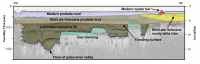
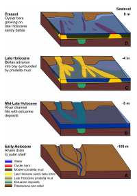 | Figure 14. Schematic block diagram showing important steps in the evolution of the Apalachicola Bay region since the last lowstand of sea level. |
 | Figure 15. Seismic profiles showing (A) oyster mounds that accumulated on an older, sandy-delta surface and were subsequently buried by younger mud, (B) an oyster bar that accumulated on a sandy-delta surface and remains exposed at the sea floor, and (C) sand waves in the eastern part of St. George Sound. The full extent of the sand waves is shown in figure 10. Vertical scales for the seismic profile are provided in milliseconds (two-way travel time) and approximate depth in meters (assuming a seismic velocity of 1500 m/s). Profile locations are shown in figure 13.
|
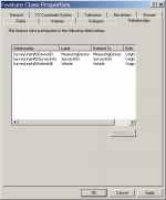
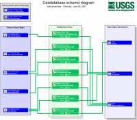 | Figure 16. Diagram of personal geodatabase showing origin and destination tables of relationship classes.
|
 | Figure 17. ArcGIS Identify results dialog box showing attributes and relationships for selected features.
|
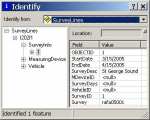 | Figure 18. An example of the information provided in the identify dialog box. |
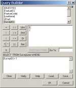 | Figure 19. Example of ArcGIS Query Builder dialog box with query syntax.
|
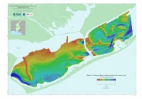 | Mapsheet 1. Bathymetry, presents a regional bathymetric model for the area using a 25-m grid cell resolution. |
 | Mapsheet 2. Sidescan-sonar backscatter, shows distribution of backscatter values over the survey area. |
 | Mapsheet 3. Surficial geology, shows the interpreted surficial geology with the locations of oyster bars superimposed on the sun-illuminated bathymetry. |
